ESA-Dresden: Sky and Background

Separation of the Noise Background from Sky and Receiver

Joachim Köppen Strasbourg 2007, 2013

Above is the background level from the empty sky measured at various elevation angles, in 2007 during the Valentine Sky Survey by Marc Cornwall. We note that the background increases towards the horizon.

These data can be interpreted in this way: The measured noise comes partly from the receiver (essentially from the first transistor in the LNB) and partly from the sky. At low elevation angles, the telescope looks through a longer column of the Earth atmosphere, and since the air is at a certain temperature, it also emits thermal radiation; the longer the column of air is, the greater is the intensity. In the simple model of a planar and uniform atmosphere, the air column increases like

1/sin(EL) However, at elevations below about 10° there is also a contribution from the radiation emitted by the ground and received by the sidelobes and the wings of the main lobe of the antenna pattern. Thus we should place less emphasis on the measurements at lower elevations.

The receiver noise will be independent of the elevation, and hence we get a simple formula for the power received by the telescope:

P = P_RX + P_sky / sin(EL) Here, P_sky is the sky background seen at the zenith (EL = 90°).

Since we measure all powers in logarithmic dB values, we have to convert them into linear power values (P = 10**(dB/10)). Then a linear fit gives the two constants P_RX = 14617 and P_sky = 2137:

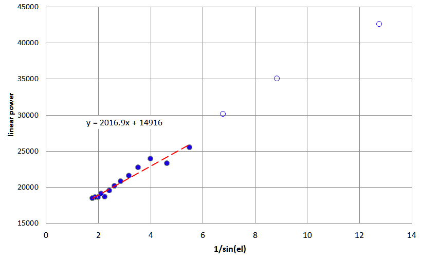
To avoid any contribution from the ground, it is better to use only data from elevations higher than 10°. This is merely a precaution, as the plot shows that those data points (down to about 5°) would also be in agreement with the linear relation ...

We could also have expressed the formula with dB values:

dB = 10*log( 10**(dB_RX/10) + 10**(dB_sky/10)/sin(EL) ) and then adjusted the values dB_RX and dB_sky until the curve computed from the formula matches the observed background values as closely as possible. This would have given the equivalent values for receiver noise dB_RX = +41.65 dBµV and sky contribution dB_sky = +33.3 dBµV. Obviously the noise we measured here is dominated by the receiver, i.e. from the first transistor in the LNB. The sky itself is of much less importance.

A simpler and quicker approach is a linear fit to the dB values, as shown here:

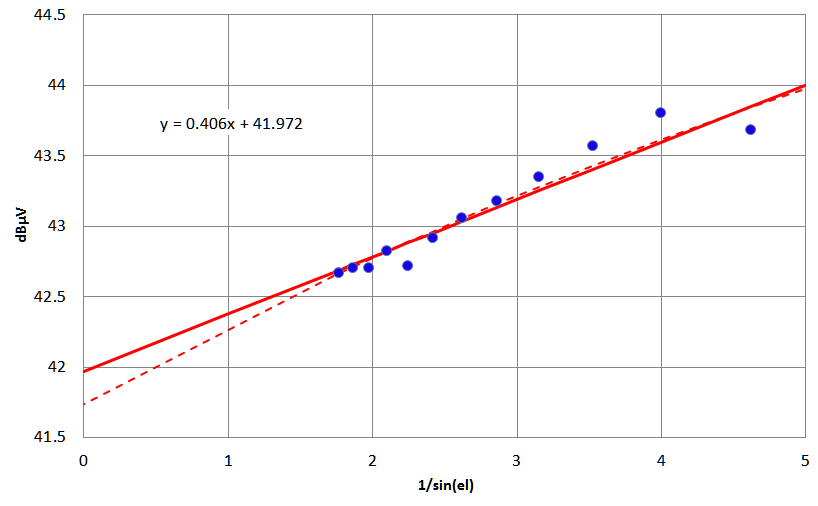
The blue dots are the same measurements as before, the full red line is the linear fit of the dB values, giving again dB_RX = +41.97 dBµV and a slope 0.406, and the broken red curve is the correct linear relation of the corresponding linear level values. As is seen here, this simplified approach is quite sufficient! The information about the sky is contained in the value of the slope.

As every position requires several minutes to accumulate a number of measurements sufficient to get a reliable average value, it is better to take measurements only at elevations that render useful information, i.e. that are equally spaced in 1/sin(el). It turns out that a sequence of 10°, 20°, 30°, and 60° gives good results.

From observations done in this manner under various weather conditions permit to compile this table below which shows that the slope is clearly related to the water content in the atmosphere. This is because at 10 GHz absorption by water molecules becomes important. Thus, clear blue skies give a flat slope, rain and thick clouds make the relation steeper. However, grey skies may only mean a thin layer of high fog, but humid polluted air shows up in the slope value:

date	RX noise [dBµV]	slope	weather
19 jun 2011	+38.62	0.127	blue sky
15 nov 2011	+39.08	0.166	fair
7 dec 2011	+38.34	0.455	overcast, rainy
7 dec 2011	+38.71	0.367	overcast, rainy
7 dec 2011	+38.64	0.346	overcast, rainy
4 jan 2012	+38.39	0.151	slightly overcast
4 jan 2012	+38.72	0.132	slightly overcast
25 jan 2012	+38.52	0.128	fair, some clouds
3 feb 2012	+39.28	0.103	clear sky
13 mar 2012	+38.47	0.105	sunny
13 mar 2012	+38.48	0.120	sunny
13 mar 2012	+38.68	0.106	sunny
16 mar 2012	+39.13	0.087	sunny
16 mar 2012	+38.96	0.120	sunny
18 mar 2012	+40.06	0.330	overcast, rain
18 mar 2012	+40.05	0.380	overcast, rain
21 mar 2012	+39.61	0.140	sunny
21 mar 2012	+39.68	0.110	sunny
21 mar 2012	+39.76	0.130	sunny
29 mar 2012	+39.62	0.109	sunny
29 mar 2012	+40.04	0.113	light overcast
27 jul 2012	+39.40	0.373	sun, clouds, humid: peak of pollution
20 oct 2012	+38.12	0.104	clear sky
18 nov 2012	+38.41	0.132	high fog
11 dec 2012	+38.77	0.117	cloudy, snow
24 jan 2013	+38.73	0.140	overcast
24 jan 2013	+38.80	0.170	overcast
24 jan 2013	+38.70	0.213	overcast
7 feb 2013	+38.58	0.160	light overcast
7 feb 2013	+38.95	0.170	light overcast
7 feb 2013	+38.92	0.162	light overcast
7 feb 2013	+38.89	0.150	light overcast

For a more comprehensive and quantitative interpretation method, see here.

| Top of the Page | Back to the MainPage | to my HomePage |

last update: oct 2020 J.Köppen