Simulation of a galaxy undergoing ram pressure stripping
Joachim Köppen Praha/Kiel Nov 2017
Some brief explanations
When a spiral galaxy travels through a cluster of galaxies, the hot gas of the intracluster medium (ICM) interacts with the interstellar medium (ISM) of the galaxy. If conditions are right, the ISM gas is pushed out of the galaxy. As a consequence the galaxy loses part or all of its gas and leaves behind a gaseous tail on its flight path.
This tool simulates this process of ram pressure stripping by a simple model. The galaxy's gas disk is divided in a number of concentric rings around the galactic centre. Each ring is represented by a single test particle which moves in the gravitational potential of the galaxy. Initially, all particles move on circular orbits around the galactic centre. The test particle is given a mass proportional to the gas surface density at the initial galactocentric radius; it is given a random position on the circumference of its ring. The action of the ram pressure by the ICM is modeled as a pulse of an additional external force which acts in a direction perpendicular to the galactic plane. Thus, we consider the situation of face-on stripping.
After a model has been computed, the positions and velocities of the particles can be inspected at a number of snapshots at different times. The user has the choice between various plots, such as plotting any two parameters against each other. These can be properties in the 3-D system of galaxy, but also 2-D views projected to the celestial sphere available to an outside observer. The user may apply rotations to the model, as to get the view of the inclined object. False colour maps are provided to give a 2-D view of the total intensity, position-velocity maps, channel maps, and the spectra of the entire object and as observed with a finite beam at some pointing position. These maps are generated by representing each ring by a number of sub-particles evenly and randomly distributed within the ring's volume.
The simulator is controlled from the page Operate.
The complete data of a snapshot may be written to the page Output in the form of an ascii text. From here it can be copied and pasted into a text editor for further use or analysis.
The controls on the Operate page are:
- The (spiral) galaxy model consists of a central bulge of stars, the disk of stars and gas, and a halo of dark matter. Each of these components is described by a number of parameters, such as its mass inside a truncation radius, and a radial scale length. Bulge and halo are modelled as Plummer spheres, the disk as a Miyamoto-Nagai disk. For comparison purposes, the user may place a point mass in the galactic centre. Because of the presence of molecular gas, the restoring force for the neutral gas is supposed to be enhanced by a factor (1 + a exp(-r/R)) as by Vollmer et al. (2001).
- Due to the ram pressure force, the test particles will be pushed away from their initial positions in the galactic plane. Depending on the strength of the force and its mass a test particle will be accelerated up to the local escape speed. Particles that escape from the galaxy are shown in the plot as red dots. Among the particles that still remain gravitationally bound we distinguish between those that remain close to the galactic plane (shown as blue dots) and those which have been pushed away (green dots), i.e. outside a cylindrical volume assigned for the galactic plane by galactocentric radius and thickness.
- The Modelling needs parameters.
The Pulse properties are:- flight speed: is the speed of the galaxy with respect to the ambient ICM. This will be assumed to be constant throughout the simulation.
- maximum pressure:
- choose between Gauss and Lorentz pulse shape, and a constant pressure ('wind tunnel').
- FWHM duration: of the pulse.
- choose between the stripped gas to follow the galaxy under acceleration by the ram pressure and to be instantly deposited in the ICM.
- number of particles: 1000 give a quick impression, 10000 make smoother curves, but 100000 are still possible ...
- snapshot interval: is the time between two snapshots.
- end time: the simulation always starts at two FWHM pulse widths before the time of peak pressure (at time=0). It will terminate at the end time, or before if the stop button is clicked.
- time step: is the stepwidth for the numerical solution of the equation of motion of each particle. For a galaxy like the Milky Way, 1 Myr is a good choice. If results look weird or if in doubt, use a smaller time step and be more patient.
- time now: during modeling it displays the time of the current snapshot.
- (vΣ)ICM: shows the current value of the time-integrated ram pressure.
- start: starts a new model. During the computation the stop button is lit red.
- stop: stops the computations.
- resume: continues with the current model. Note that a model can be extended by specifying a larger value for the end time.
- Display controls:
- inclination YP, ZP: are the angles of rotation around the YP and ZP axis of the observer's 2-D view. The observer's image has XP and YP as the horizontal and vertical axes, ZP is the direction along the line of sight.
- for the spectrum at a position these controls are visible:
- point at XP, YP: these are the coordinates of this position. The point is marked as a plus-sign in the total intensity map, channel map, and the XP-YP plot.
- antenna HPBW: also, one can specify the HPBW within which all particles are included for the spectrum.
- for the position-velocity map these controls can be used:
- point at YP: The map is done for a fixed position in YP. [no control of position angle yet :-)]
- antenna HPBW: also, one can specify the HPBW within which all particles are included for the spectrum.
- for intensity map and channel map
this control is avilable:
- antenna HPBW: the maps also take into account a Gaussian antenna pattern.
- number of map/histogram bins: maximum is 100.
- X, Y: if one has chosen all other plots one can select the parameters to be shown as abscissa and ordinate.
- Set range: In order to use values for the X and Y ranges more convenient than the standard value, enter the wanted minimum and maximum values in the two fields and click the circular radio button to show the same plot with the new range. This applies to all types of plots.
- colour bar (for the false colour maps): one may choose between:
- linear rainbow: between black/violet = 0 and red/white = 1
- rainbow-2: with larger emphasis of high intensities. The colour bar at the right rim indicates the colour distribution between 0 and 1.
- rainbow2: with stronger emphasis of low intensities
- rainbow4: with even stronger emphasis of low intensities
- rainbow8: with very strong emphasis of low intensities
- log rainbow 0.001-1: logarthmic between black/violet = 0.001 and red/white = 1
- output this snapshot: the current snapshot's data will be written as an ascii table on the Output page
- time ← →: are the controls to navigate among the snapshots: either by the buttons with arrows or entering the snapshot number in the text field between them. The proper time of that shapshot is displayed at right.
- had one chosen the channel map these controls are visible: radial velocity, channel ← →: are the controls to navigate among the radial velocity channels. Δv is the width of the radial velocity window. Use the buttons with arrows to step forward or backward by one channel, or enter the desired central value for the radial velocity in the text field between them.
- Mouse position: displays the coordinates of the present position of the mouse. In the false colour maps it also shows the actual surface density as well as the value relative to the image's maximum value.
The user may choose among these plots:
create a model: galactic X-Y plot: This is the default plot when the simulator is loaded, and also the recommended plot to watch the progress of a simulation. It shows a face-on view of the galaxy. First, all particles are blue, because all are well inside the volume assigned for the gas disk. In the course of time particles turn green, as they are pushed out of the disk, and evenually some appear in red when they have reached escape speed. For better visibility, in models of more than 5000 particles only one tenth are displayed.
all other plots: here, one may plot any two parameters against each other, whether they are sensible choices or not :-). One may follow the evolution of the model calculation for instance by plotting the distance from the rotation axis as a function of time ...
total intensity map: is a false colour representation of the density of particle masses in the observer's XP-YP view. Since the mass of a particle is proportional to the surface density at its initial position, this map shows an image of the surface density of HI (in units of MSUN/pc²), and thus of the brightness distribution in an image taken in the HI 21 cm line. The map can also be computed for a non-zero HPBW of the antenna, but one should exercise a bit of patience for the image to appear.
position-velocity map: is a false colour representation of the surface density in the XP-VRAD plane (in units of MSUN/pc²) at a 1 kpc wide strip at constant YP, which corresponds to a horizontal cut in the total intensity map [use of an arbitrary position angle is under consideration]. Note that using a non-zero HPBW of the antenna requires some extra time for the image to appear.
channel map: false colour map of the surface density in the XP-YP plane of particles whose radial velocity is near the specified value. With a non-zero HPBW of the antenna the the image needs some more time to show up.
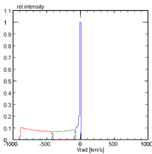
total spectrum: shows histograms of the radial velocities of all particles of the three types. The asymmetry of the sum spectrum with respect to the systemic velocity is computed from the fluxes integrated over the blue (= left) and red (= right) sides. The ratios r/b and (r-b)/(r+b) and max(r/b, b/r) are displayed.
spectrum at point (XP,YP) with HPBW: is the histogram of the radial velocities of all particles whose projected position (XP,YP) is within the HPBW of the selected point. The asymmetry of the spectrum is displayed, as above.
The variables of the model are: Note that the variables are a mixture of various types, and therefore it may not be too meaningful to plot certain parameters against certain others ...
- time: is relative to the instant of maximum pressure.
- ram pressure: permits to plot the dependence of e.g. gas mass fractions as a function of the instanteous ram pressure.
- time integrated ram pressure (vΣ)ICM: permits to plot the track in the (vΣ)ICM-ram pressure plane.
- - - - - - - - -
- galactic X,Y,Z: the position of the particles in the galaxy's coordinate system.
- distance from rotation axis:
- initial distance from rotation axis:
- galactic VX,VY,VZ: the velocity components in the galaxy's system.
- speed:
- radial speed: the component radially away from the axis of rotation.
- tangential speed: the component parallel to a circular orbit.
- gas surface density: in the plane of the galaxy, when viewed face-on
- tail surface density: this is an estimate which applies onlly along the axis of a tail viewed from the side (at incl.YP = 90°)
- total energy:
- angular momentum density: carried by each ring
- - - - - - - - -
- observer's projected XP,YP: the positions of the particles as seen in an image by the observer.
- radial velocity: the speed along the line of sight from the observer.
- - - - - - the ordinate has these additional variables - - -
- ram pressure: to be plotted as a function of time
- remaining gas mass fraction: can be plotted against time or ram pressure. This is the fraction that keeps close to the galactic plane. These particles are shown as blue dots.
- kicked gas mass fraction: is from particles that have been pushed out of the galactic plane, but remain bound to the galaxy. Shown as green dots.
- kicking radius: the innermost distance of green particles, i.e. the outer radius of the particles that remain in the disk.
- stripping radius: the innermost distance of red particles, i.e. the outer radius of the particles that do not escape from the galaxy.
- mass loss rate: of the gas that is gravitationally bound to the galaxy.
- stripped gas mass fraction: is from particles that escape from the galaxy (shown as red dots).
- gas deficiency: = log10(initial gas mass/final gas mass)
| Top of the Page | back to RPShome | Java Applets Index | JavaScript Index | my HomePage |
How to ...
- ... check basic properties of the galaxy model
The characteristics of the galaxy which essentially determine the outcome are the rotation curve and the initial gas surface density profile. Both can be inspected directly by choosing these X/Y parameters. After making any parameter entry, run the model for a few time steps.

- ... compute a model
Running the default model gives this view of the final state of the galaxy, at 75 Myr after the maximum pressure of 10800 cm-3(km/s)² from a 25 Myr long pulse with a flight speed of 1300 km/s: Blue dots show that in the inner part of the galaxy some gas is still close to the galactic plane. Green dots mark the particles which are pushed out of the disk, but remain bound to the galaxy, while red dots show particles that are escaping. The false colour map shows the total intensity as would be seen if the galaxy is viewed face-on in e.g. the HI 21 cm line.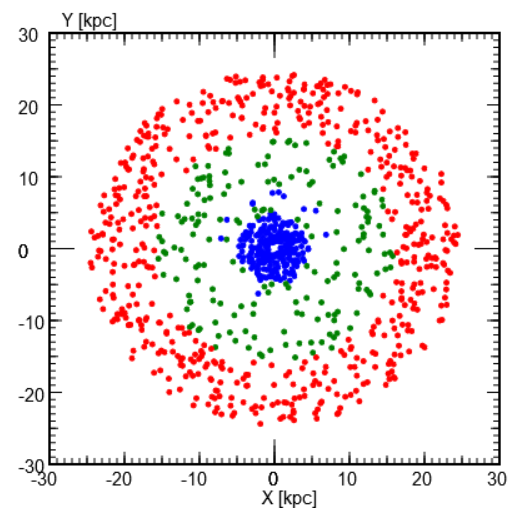

- ... follow the evolution
If one chooses to plot the distance from the rotational axis (named 'rho') for all particles as a function of time, running a model will show when the gas at various radii is perturbed and eventually leaves the galaxy. The perturbed particles also move radially. Both escaping and kicked particles start to move outwards some time after the peak pressure.
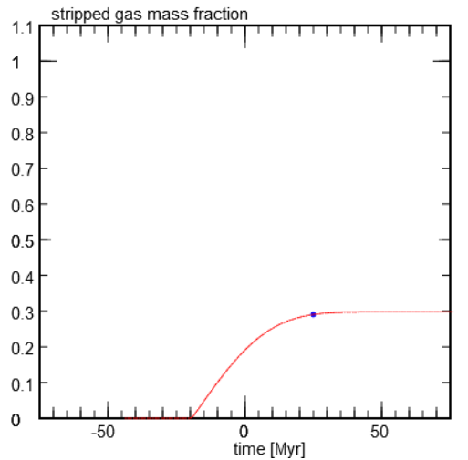
Similarly, one may chose to watch the growth of the stripped mass fraction with time. During the computation, the small blue dot indicates the current time; after the model is complete, the dot on the complete curve indicates the selected snapshot.
- ... look at the spectrum
The left hand plot depicts the total spectrum (with 40 bins) at the last snapshot of the default run. Blue, green, and red curves show the contributions by the particles that remain near the galactic plane, the ones pushed off the plane, and the stripped particles, respectively.
The spectrum (100 bins) depicts the situation at some earlier instant.
- ... look at a tilted galaxy
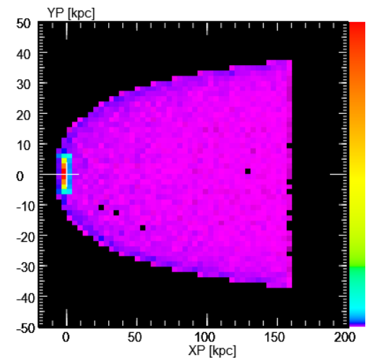
The left hand map of the total intensity was done with 10000 particles, with inclinationYP = 60°, inclinationZP = 50°, and setting the ranges for both axes to convenient values.
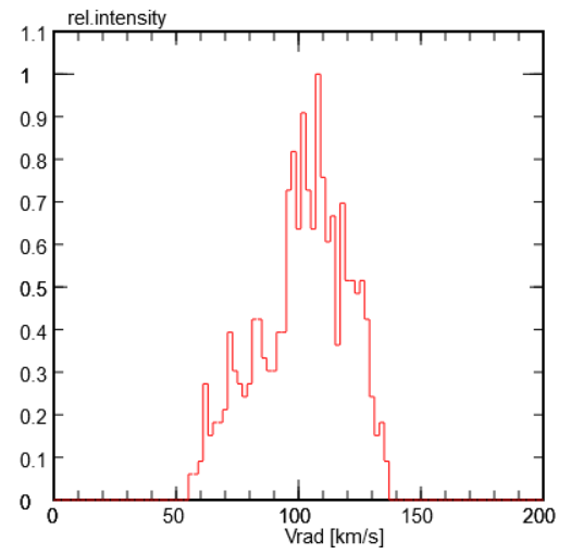
The spectrum is taken at the position indicated by a white cross in the map on the left, and shows the line profile at the start of the tail for HPBW = 2 ° (From a model with 100000 particles).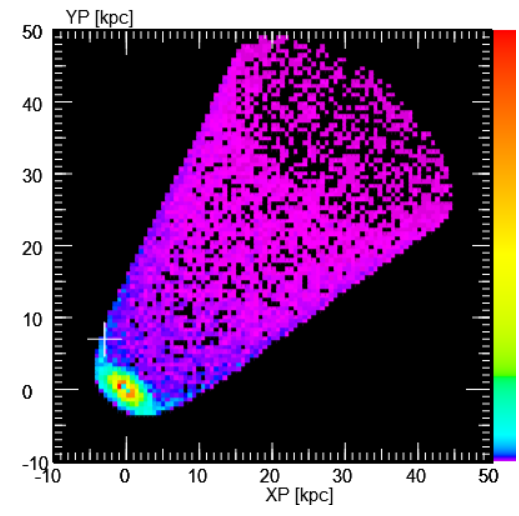
- ... inspect the gas tail
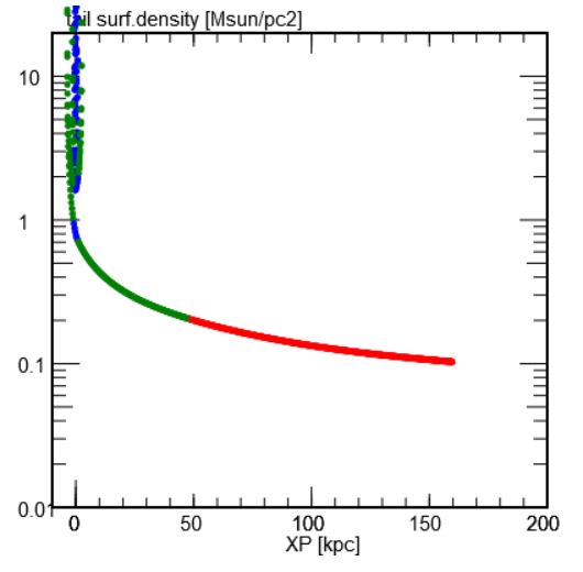
It is important to keep in mind that each test particle represents an entire ring. The map on the left shows the positions of each particle, but also its state (in the disk, kicked or escaping). The intensity map in the middle is constructed by representing each ring by a number (100) of sub-particles of correspondingly smaller mass which fill the ring's volume. Since they are randomly generated, the map is a bit noisy; their number was chosen to give a short response time of the tool. The plot on the right displays the surface density in the tail, viewed from its side, as a function of the distance from the galaxy.
- ... get smoother snapshots:
Suppose we wanted to use a snapshot of a simulation as a model for another purpose, but this model should less noisy than the original snapshot. Instead of making a model with a larger number of particles, we can make use of the fact that each particle represents an entire ring in the x-y plane, and generate particles at other positions of the same ring by making use of rotational symmetry:
From a particle at (x, y, z) with velocity components (vx, vy, vz) (with r² = x² + y² and the speed in radial direction vR = (x*vx+y*vy)/r) we create other, equivalent particles of the same ring by picking various azimuthal angles φ and compute their positions (r cosφ, r sinφ, z) and velocity components (-vR sinφ, vR cosφ, vz) - ... look at the limiting cases
The left hand plot shows a model in the long pulse limit: the duration of the pulse 1000 Myr is much longer than the period of oscillations perpendicular to the galactic plane (between 20 and 200 Myr for this model galaxy). As a consequence, all particles which are pushed away from the disk plane eventually are stripped. One notes that during their acceleration they also move radially outwards and escape at greater distances from the centre than their initial positions. There are no particles that will later fall back to the plane.
The plot at right displays a model in the short pulse limit: with a pulse duration of 1 Myr all particles receive the available momentum. Because of their lower surface density, particles of the outer rim are quickly pushed to escape (red area) at their initial distance from the centre. Quite a while after the pulse the particles at more inner positions leave the galactic plane, performing vertical oscillations about the plane (green area). They represent extraplanar gas that eventually falls back into the disk.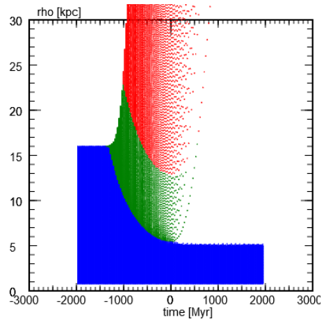

Mass [MSUN]
Bulge ( = Plummer sphere)
Mass [MSUN]
Radial scale [kpc]
Truncation radius [kpc]
Stellar disk ( = Miyamoto-Nagai)
Mass [MSUN]
Radial scale [kpc]
Truncation radius [kpc]
Thickness [kpc]
Gas disk ( = Miyamoto-Nagai)
Mass [MSUN]
Radial scale [kpc]
Truncation radius [kpc]
Thickness [kpc]
Restoring force enhanced by molecular phase
Enhancement factor
Radial scale [kpc]
Dark matter halo ( = Plummer sphere)
Mass [MSUN]
Radial scale [kpc]
Truncation radius [kpc]
Galactic plane
half thickness [kpc]
radius [kpc]
Pulse properties
flight speed [km/s]
Max.pressure [cm-3(km/s)²]
FWHM duration [Myr]
Modelling details
no. of particles
snapshot interval [Myr]
end time [Myr]
time step [Myr]
time now [Myr]
(vΣ)ICM [Msun/pc² 1000km/s]
Display
inclinationYP [°]
inclinationZP [°]
point at XP YP
Set range: ...
Set range: ...