Calibraton of the Data

Joachim Köppen DF3GJ Kiel/Strasbourg/Illkirch Spring 2004

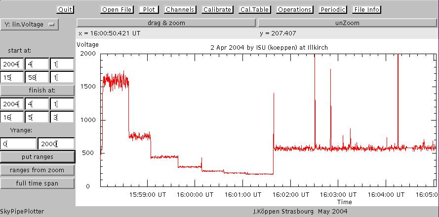
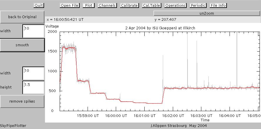
First, it is useful to remove the spikes and also to smooth out the fluctuations from the noise. The technique is to check every datum whether it lies above a straight line connecting data 10 pixels apart ("width"); if it does so by more than a factor (1+height) of the current y-value, the datum is replaced by the value predicted by the straight line. Smoothing is done simply by averaging over the 10 pixels left and right of each pixel. One fiddles with these three parameters, until one obtains what one accepts as a nice result, shown in the red curve, with the original data in grey:

Then we rather take the logarithm of the ordinate values, as to better aim the low level calibration steps. We know that the calibrator had a maximum noise level of +34 dB over thermal noise of 290 K, thus corresponding to a temperature of 736 kK. Each step is 5 dB (a factor 3.16) lower in temperature than the previous one. We start the calibration by clicking the "begin cal." button, then we click with the mouse on each step which is marked with a blue dot:

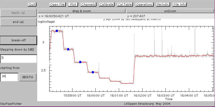
and after we finish by clicking "end cal." we get the data in terms of dB over thermal noise:

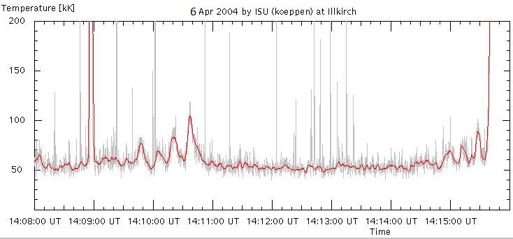
We now can display the y-values in real temperatures

from which we read off that the afternoon noise level at ISU was about 120 kK.

After calibration which is kept inside the program, we can read in the interesting part of the observations and display it in proper temperatures: