Our New Software for the ESA-Dresden Radio Telescope

Joachim Köppen Kiel/Strasbourg 2009

• How to start
• Operating Page
• Skyview Page
• Spectrum Page
• Scan Page
• Map Page
• Pos.Calibration Page
• Settings Page

This is not a complete tutorial, but rather a brief summary of the steps to make a simple solar drift scan observation:

• start the program by double clicking the icon on the desktop
• and you will see the Operate Page
• click on Startup System, and you should read in red letters "port 2 is now open for Radio": this means all is well!
• also, the current position of the telescope is shown in the top centre.
• click on goto Calibrator and the telescope will move to the calibration source
• click on Start to commence measuring and recording. This is also indicated by the green colour of the Operate button
• the receiver takes one measurement every 2 seconds, and the result (in dBµV) is displayed as a number, as a coloured bar at right, and as a red curve in the central plot.
• after about two minutes to get a nicely long block of calibrator signal, click on Sun now which will display the present position of the Sun
• click on Goto to move the telescope to that position, and the signal should go up ...
• However, because of the finite accuracy and stability of the rotator system, in general you will not get the maximum signal! Move the antenna manually a bit (+/-1° or so) around to really get the highest signal. Sometimes, a short tap on the rotator controls has a great effect, but no change in the displayed position! But if you notice that the current position is somewhat different from the true solar position, keep these offsets in azimuth and elevation in mind for later use:
• now click on Sun+15m and then on Goto to move to the position where the Sun will be in 15 minutes. But if you had noticed any offset, correct the position accordingly!
• Then simply wait and hope for the best, that the Sun will indeed pass centrally through the main lobe!
• After the maximum signal, wait until the signal has gone down to the value of the empty sky, and has become nicely constant.
• click on goto Calibrator and take another 2 minutes calibration signal.
• you can Stop the run, and adjust with the sliders at left the scale and the value of the vertical axis of the plot to suit your needs best, and then you can continue by clicking on Resume.
• If you want to finish or break off this observation run, click on Stop+Finish. After that, you can only start a new run which is recorded in a different file.
• The data files are normal *.txt files, in the folder (JKStuff) where the Java class files reside. They are chronological labelled, e.g. UT0904011400.txt for the run started at 14:00 UT on 1 April 2009.

• To close down, click on Shutdown System and then on Exit, or simply on Exit

• Green: an observation run is going on on oone of the pages
• Yellow: a mild warning, for instance that it would take some time to complete the observing task
• orange: a severe warning, such as that the expected observation time would take VERY long, or that the requested position is out of the permitted range. In the latter case, the telescope will not execute this move.
• red: the expected observation time is outrageously long: don't be such a fool!

This is the main page of the software, and thus seems to have a frightning number of controls ... It shows a simulated drift scan observation of the Sun, preceeded by a flux calibration. The structure of this page is quite simple:

• the top row of buttons allows to navigate to the different pages which permit a variety of observational procedures
• below that is the geographical position of the station and the current time
• the button Shutdown System (initially: Startup System) had started the communication with the rotator controller interface and the receiver. To its right, messages will be displayed, as well as the information whether we are running a "Simulation" or "Real Life"
• the next row of buttons deals with certain useful positions:
  • goto Calibrator will move directly to the calibration source
  • goto Astra 1 will move directly to that satellite
  • Sun now will display the current position of the Sun, but one has to execute that move by clicking on Goto
  • Sun+15m as above, but for where the Sun will be 15 min from now
  • Moon now as above for the Moon
  • Moon+15m as before, for the Moon
• the current Position are given in true Azimuth and Elevation angles. For internal use, and for comparison with the Dresden software, we also display 'our' values at the right.
• the next line gives the Fields where we may enter the true AE/EL where we want to go next. This move is executed by a click on Goto.
• next are information necessary for the observing run:
  • we can enter the freq. [MHz] (in integer values!)
  • and set the sense of Polarization
  • Also, we may specify whether we want to record on file the data average over a number of measurements. Normally (enter: 1) every datum is stored, but for long duration observations it may be useful to average over a number of data. This will also make the files shorter ... Irrespective of this setting, the plot will show every datum.
  • single measuremt. takes a single reading of the receiver, which is displayed and plotted, but not recorded in a file.
• the last row of buttons permits to control the observation run:
  • Start starts with the regular measurements (one every 2 seconds) which are recorded on file
  • Stop interrupts the measurements. Then one may adjust the level and the range of the ordinates in the plot!
  • Resume continue with the present run
  • Stop+Finish terminates the present run. Next run has to be restarted and is written in a new file
  • power here the current measurement is displayed in numerical form
• at the lower part, there are two graphical displays of the data: a chart-type plot which shows the data so far recorded, and a bar representing the current signal strength. The range and the level of either graphs can be adjusted by using the sliders to their left. The bar graph can always be adjusted. The chart, however, can only be altered when the measurements are not running.

This page gives a view of the sky as it would appear if we looked down on our observing station. It shows

• the blue area is the permitted area for the antenna rotators. We should not try to goto elevations higher than about 55°, because of mechanical constraints ... if one operated the rotator beyond that limit, it would slip on the elevation axis, and one would have to recalibrate the positioning system ...
• the black shapes near the horizon are nearby buildings, which we can use as calibration sources. Our standard source is maked with a violet cross
• the blue curve denotes the Clarke belt of the geostationary satellites
• the yellow dot is the Sun, the blue dot the Moon
• the red cross is the current position of the telescope
• we had also clicked the mouse on that position, and thus it is displayed at upper right
• the yellow Goto button permits to move the telescope to that position
• on the upper left, the time is displayed
• the three yellow buttons permit advance or set back the time by 1 hr (per click) and to show the sky situation. In that case, the time will be backlit with violet. The button now resets back to the current time

• Start freq.[MHz] is the lower frequency (integer values)
• End freq.[MHz] is the upper frequency (integer values)
• Freq.step [MHz] is the step (integer values only!)
• No.of samples at every frequency we'll take the average over this number of measurements
• the orange field indicates that with the specified parameters this scan would have taken 1 hour, which is rather long, and certainly too long for a moving source like the Sun and the Moon!
• Start commences the spectral scan
• Stop interrupts it - and hence allows readjustment of the chart's range
• Resume continues with it
• when the spectrum is finished, both Stop and Resume buttons are disabled

• Start Position are given in azimuth and elevation
• End Position likewise
• No.of steps: for our rotator system it does not make sense to have steps finer than about 1°! This must be taken into consideration
• No.of samples at a point the recorded and displayed measurements will be the average over this number of measurements taken at each position
• the yellow field indicates that with the specified parameters this scan would have taken 16 minutes, which is a bit long, therefore the mild warning in yellow! If we had done this in Real Life, the Moon would have gone away, and hence we would do such a scan better with a smaller number od samples or step!
• Start commences the scan
• Stop interrupts it - and hence allows readjustment of the chart's range
• Resume continues with the scan
• when a scan is finished, both Stop and Resume buttons are disabled

This page allows to make maps or images of the sky. However due to the finite accuracy and stability of the rotator system, this feature cannot work in a satisfactory way!. Here is shown a simulated image of the Sun. The controls are

• Centre Azimuth, Elevation When you access this page, the current position is taken as the centre of the map. But you can modify these values as you like.
• +/- range specifies the span in horizontal and vertical direction that the image should have. A value of 3° means that the image size will be 6° by 6° in the sky.
• no.of points tells with how many 'pixels' you want to cover the spans in either direction. The reddish background of the fields is to indicate that the steps in azimuth and elevation would be less than the 1° that our rotators can manage! We should never attempt that in real observations ... apart from the fact that the actual positions may differ from the requested ones, because of the finite accuracy of the positioning system, mechanical backlash, etc. It will be investigated, how well our real system can cope with this task ...!
• no.of samples tells over how many measurements we shall average at each position.
• the orange field indicates that the expected observation time is 1 hr, and thus will require some patience
• the false colour image shows the result. The colour and the range of colours can be adjusted by the two sliders on the left hand side, and the correspondence of colours and values can be read at the left most colour bar. These adjustments can be made during the ongoing observations
• Start commences the mapping
• Stop interrupts it
• Resume continues with the mapping
• when a scan is finished, both Stop and Resume buttons are disabled. The telescope will then be at the position in the upper right hand corner

From here, we can inspect the correspondence of the true sky positions with 'our' coordinates, which are the ones with which the rotator controller works. Since our telescope has been placed on the roof without going through a laborious procedure to align it accurately to the true north, we use the positions of geostationary television satellites to do this alignment by software, as explained here. This is how to do it:

• at the left, there are pairs of fields for the measured positions of 22 satellites. The fields where the next data will come in are highlighted in turquoise. However, it is possible to modify the data entries ...
• one can maneuver up and down by next Sat. and previous Sat., or start again
• The central plot shows these measured positions as blue dots, in comparison with the red curve of the Clarke Belt, the locus of geostationary satellites seen from our location. A blue cross indicates the current position of the telescope.
• switch the receiver to its spectrum analyzer mode ("Analyze", "SAT") and move the antenna manually by the keys of the Yaesu rotator controller
• when a satellite comes into view, one can see the channel structure in its spectrum, for example:
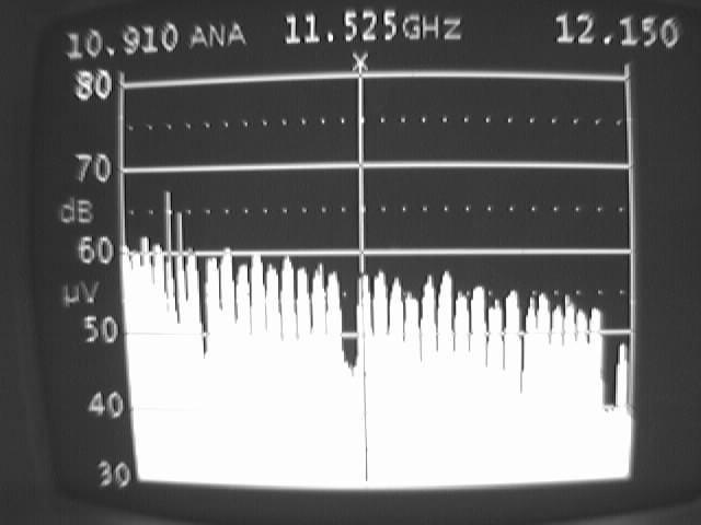
• when you have found the position which gives the strongest signal, click on accept data. This will add this satellite -- we do not need to bother about its coordinates -- and display it on the plot
• this procedure is repeated as often as you want. You may fill all the fields or simply take four or five strategically placed satellites
• then one plays with the four numbers at lower right, such as AZ offset, until one finds a good match of the positions and the Clarke Belt.
• when you are happy with the result, click accept fit which will from now on apply this transformation to the positions. It also stores the values on hard disk, as to be read the next time you startup the system.
• when in doubt about the positions -- perhaps after a big storm -- goto a satellite (e.g. goto Astra 1) and check whether you still get a maximal signal. Because of this, it is recommended to always 'park' the telescope on that satellite, so we can easily verify that everything is fine.
• whenever need for recalibration of the positioning system arises, with four nicely placed satellites one can re-establish calibration within a few minutes!
• plot is pretty superfluous

This page is normally without any importance to the observer, but it may be useful when one needs to check the state of the program. It shows all the parameters that are read from the initialization file edtini.txt at the start of the program and written to it when exited. One may change the settings, and store them for the next startup. Some comments:

• Accept and Save Settings is used after one has modified one of the enries
• Rotator control port should be "COM1" and "9600" Baud. But we can set it to "simulated"
• Receiver control port should be "COM2" and "19200" Baud. But we can set it to "simulated"
• Output format is the format for the file where the measurements from Operate page

  and some temporary features (for tests during development only):

• Sim is fast here we can slow down the simulation to resemble better the real observations
• pos/meas.steps DON'T EVER TOUCH THESE VALUES ...

| Top of the Page | Back to the MainPage | to my HomePage |

last update: 1 April 2009 J.Köppen