How to Determine the Thickness of the Galactic HI Disc
Marissa Rosenberg, Joachim Köppen Strasbourg 2010
If we had eyes to look at the sky in the light of the 21 cm line of neutral hydrogen
we would see like in the all-sky image below (from National Radio Astronomy Observatory
/ Associated Universities, Inc. / National Science Foundation) that the emission
in strongly concentrated along the great circle of the Milky Way: The hydrogen gas is
essentially found in the Galactic Plane.
It forms a rather thin disc, a bit like a pizza, with a diameter of about 30 kpc and
a thickness of about 200 pc. The gas is in the form of clouds (with a mean density of
about 1 atom per cubic centimeter and above) that fill the vast space between the stars.
It is from these clouds that eventually new stars are formed when such a cloud becomes
massive and compact enough to be able to cool and form molecules, and finally collapses
under its own gravity.
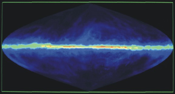
The gas disc is substantially thinner than the disc in which the stars are located. From
the above false-colour image we also get the impression that the thickness is not the
same in all directions. For example, towards the Galactic Centre - in the centre of the
image - it looks thinner than in the direction of the anti-centre. Let us measure the
thickness of the gas disc, and find out more about the gas in our own Galaxy. Below we
describe how to do it as a workshop activity:
Objectives:
- Become familiar with using a radio telescope
- Understand how radio observations can teach us about our Galaxy
- Derive the thickness of the Milky Way’s gaseous disc
Materials:
- ESA-Haystack Radio Telescope
- Computer with JKSRT3 software to operate the radio telescope
- Computer with Microsoft Excel for the analysis
Observational Procedures
Once you started up the system, as described here you
are ready to observe. Here we will expose you to two different types of
observation. First it is important to try the manual version. It is good to know
what you are looking for
and you will get a real feeling of what it is like to use a telescope. We hope
that seeing how easy it is to use will motivate you to do some of your own
observing. We also want to provide some hints on what you should be looking for
while you’re observing. First, watch the waterfall plot. The variation you see
between each line should be slight and is due to the fluctuations of the noise in
the signal. You may click on the yellow fields to adjust the range of the values
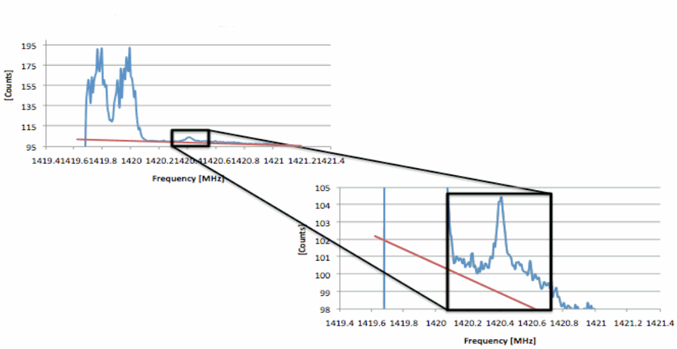
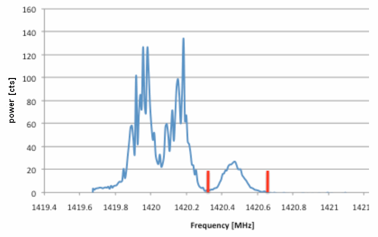
represented by the colours. Since the galactic emission is concentrated to a
narrow frequency range, you should be able to discern eventually a vertical band
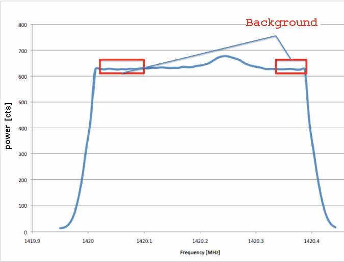
of slightly higher signal. This is also seen in the frequency plot to the upper
left: the black curve shows the current spectrum, the red curve is the accumulated
one, so that after a while the galactic features would become more distinct.
After you had tried the manual observing, we will encourage you to run batch files
while you are in class or doing other things. This will allow for much easier,
less tedious data acquisition and hopefully permits you to accumulate as much
data as you may need.
Manual Observations:
- Find the four places along the Galactic Plane labeled G20, G90, G150, and G180,
indicating their galactic longitude. You will notice there are multiple other
locations associated with them (G20.5, G90.10n, etc). These are the different
galactic latitudes at which we will make observations (above and below the Plane).
- Find which point is currently visible and not close to the horizon.
- Make sure that your frequency is centered at 1420.4 MHz and your width is 1500 kHz
span. Also, if not already done, plug in the PointCorr:
Az =-0.5 El = -3.5 which are corrections necessary for the proper positioning
in the sky.
- Move the telescope to G__.0, with __ indicating what ever longitude you had
chosen, by clicking on that point. It is good to start with the position in the
Plane, as the signal is strongest. The name of the source will be displayed
on the right hand panel, and the telescope will execute the move. The actual
position is displayed on the top right, with a background that blinks red
(while moving in azimuth) and blue (elevation).
- When it is finished moving, have a look that the galactic feature is somewhere
in the middle of the range. If not, you can change the central frequency by
entering it in the corresponding field and hitting the return key. At the lower
right, an appropriate message should appear in blue letters.
- Press the Record button and time this observation for about 5 minutes.
- Everytime you give a command, record it in the logbook, as well as
any notes that you may have on the spectrum.
- After 5 minutes, continue recording but move the telescope to the next
latitude position
- Repeat steps 8 and 7 for all the latitudes
- After your last observation, stop recording by pressing the Record
button again.
- in case neither you nor someone else wants to use the telescope,
stow it by pressing Stow on the top bar. Then shut down the
system as described here.
- You find your recorded data in the text file at: C:/SRTcassi, named:
year/month/day/time.txt for example: 1004141630.txt if I observed
starting at 16:30 on April 14th 2010 (all times are given in UTC).
Copy the file to your USB stick or flash drive to transfer onto your
computer.
Batch Observations:
- Find which galactic longitudes are visible.
- Click cmdfil and open the .txt file for whichever G coordinate you
want to observe. If you want to observe G20, open G20.txt.
Each batch file will go from G__.15n to G__.15 observing each latitude
for 500 seconds (to be tried and decided).
- In your first batch observations you might want to follow what is going on
for a while. As each position takes about 8 minutes, you have time to observe
how well the features in the red curve build up. The final spectrum will be close
to what you will obtain in your analysis.
- After about one hour the batch is completed, you can find the file
in the same place as above, step 12.
Analysis
Basic Operations
- To import your text file to Microsoft Excel, go to: File -> Import->
Text File -> Select your Text File -> Delimited Text file ->
Delimiter is spaces -> Finish
- Each row represents a single spectrum taken by the telescope at a
certain time instant. The columns from left to right represent: Time,
Azimuth, Elevation, offsets in azimuth and elevation, velocity with
respect to the Local Standard of Rest (LSR), the first frequency in
the spectrum, the frequency increment, an integer number indicating
the frequency mode, the number of frequency points in the spectrum,
followed by the flux at the first frequency all though to the flux at the
last frequency.
- It is very convenient to separate each block of data corresponding
to a latitude value into its own worksheet. If you observed from b=-15°
to +15°, you should have 7 separate worksheets.
Treatment of Each Latitude
- Let us start with one worksheet: Insert at least 4 rows in between the
top of the page and your first row of data.
- Insert two columns in between K and J.
- Above the first flux measurement, start an array that tells the frequency
for each column. You can do this by starting with the frequency given in
column G and adding the given increment (column H) to each subsequent
column.
- Next, let us examine the time-averaged spectrum: Create another
array below the frequency array, and put in the averages of the values of
the fluxes measured during the time we stayed at this position. Now
plot frequency versus flux and inspect the results.
Removal of the Baseline
- As we had noticed in Step 7, there is a high level of background noise in
our measurements, mainly from the noise produced in the electronic devices
of the receiver itself. This is called the baseline, above which any genuine
external emission is seen. As the noise is fairly independent of frequency,
we can subtract this background, either as a constant value or by assuming
that is a straight line, so that the baseline flux varies linearly with frequency.
- Using the plot we made in Step 7, select left and right of the feature of interest
an empty spectral portion and take average values from both sides.
The graph below shows an example where it is easy to find suitable portions to
define the baseline, which is rather constant. Put this average value in some
convenient cell next to the averaged spectrum.
- Below the time-averaged flux array, create an identical flux array with the
baseline flux subtracted from the original flux values. Now plot these reduced
fluxes against frequency, like in Step 7. In this plot the flat portions of the
spectrum should be close to zero. If not, you can adjust your choice of the value
for the baseline flux.
- If you notice that the flat and low portions of the spectrum do not meet the
horizontal axis in the same manner, you have to deal with a sloping baseline.
You must model a line using this equation:
F(f) = Fa + (Fb-Fa)/(b-a)*(f-a)
where you estimate the frequencies a and b and the
fluxes Fa and Fb that best fit the background near the galactic
feature. Make sure that it fits the whole profile as well as a zoomed in picture
of the galactic feature.
Finishing
- Repeat steps 4-11 for each galactic latitude (b)
Determination of the Vertical Profile
- Open a new Excel worksheet and copy and paste the Frequency and Flux–Baseline
fields from the top of each measurement. When you paste be sure to
“Paste Special -> Values”.
- We essentially need to integrate the total flux received for each observed
latitude. If we plot the total flux by the galactic latitude we should see a
peak of total flux when looking directly in the Plane and it should decrease
as we look further from the plane. To integrate the flux, SUM the flux
values at each time-averaged spectrum, ignoring negative values. Make sure that
you integrate only over the galactic feature, and not include any in-band
interference signals. The red tick marks in the figure below give an example of
how to place the integration limits. On the left hand side you see the strong
interference we had named the “Twin Towers”. Notice how the genuine galactic
emission was dwarfed by them.
- Now let's plot the total flux as a function of latitude. Do your results match
the expected outcome?
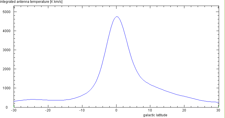
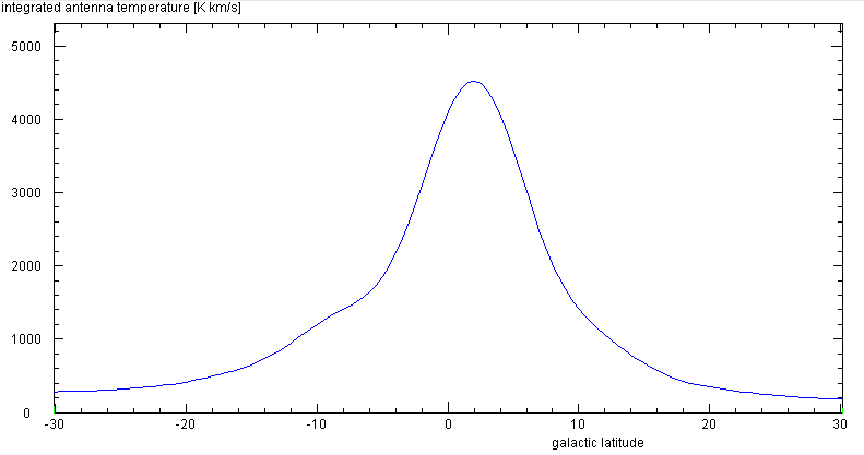
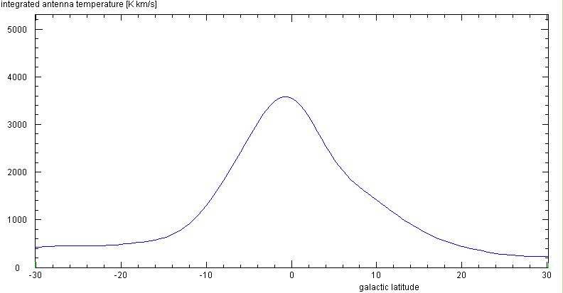
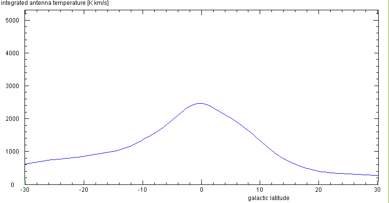
From the Leiden/Dwingeloo Survey of the HI disc - done with a 25 m diameter radio
telescope - one obtains these vertical profiles, after degrading the angular
resolution to 6°, the HPBW of our telescope: l=20°
90°
150°
and 180°
Interpretation and Modeling
We may interpret the obtained vertical profiles in various ways:
- The simplest approach is to determine the Full Width at Half Maximum (FWHM).
We measure it, as the name implies, by finding the maximum flux and then the
two galactic latitudes where the flux is half this level. The span in latitude
is the FWHM, in units of degrees.
- We may compare this value with a very simple model which consists of assuming
that the gas density in the disc decreases like an exponential function, both
radially outward and vertically with distance from the Plane. How quickly the
density drops, is described by a radial scalelength and a scaleheight, respectively.
The JavaScript tool below computes the expected FWHM observable at any galactic
longitude, either as the true distribution or as seen with a telescope with
a given HPBW. Enter the galactic longitude of your vertical profile in the
field gal.longitude and the HPBW = 6°. The plot on the right hand side shows
this vertical profile. Vary the scaleheight until you obtain the same FWHM
that you had found. What value do
you get? How does this compare with the "textbook value" of 0.14 kpc which
is often used for modelling the gas disc?
- When your data is nice, and maybe you had obtained a profile with latitude
step as fine as 2°, and maybe you followed the profile out to latitudes as
high as 30°, it may be worth looking at the entire profile: is the profile
symmetric? What kind of function could best describe it? Compare it with
a Gaussian or an exponential function with suitable parameters? Would that
reproduce the shape of the profile?
Modelling tool for the Galactic Disc
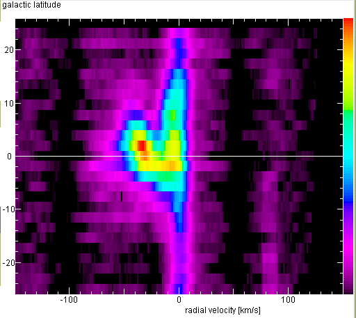
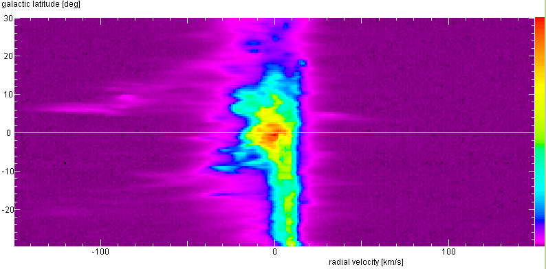
Latitude-Velocity Diagrams
When making the vertical profiles, we throw away the information from the radial
velocities. Since the frequency of a feature in the spectrum relates to the radial
speed with with this packet of gas moves away from us or moves towards us, we can
learn also something about how the gas motions in the disc: The easiest way is to
make a map - similar to the waterfall plot:
- It is best to open a new Excel worksheet and copy and paste the
Flux–Baseline fields into a number of rows which you had labeled with
each latitudes (again, when you paste be sure to “Paste Special -> Values”).
- in the row above this block you put consecutive numbers which indicate the
number of the frequency
- then grab the entire data block and make a surface plot. As with the waterfall
plot, you can change the number of color levels and the colours themselves
to your taste ... Since the higher frequencies means more negative radial
velocities, it is good to invert the sense of the frequency axis.
- The result would look like this (our data for l=150°, done with latitude
steps of 2°)
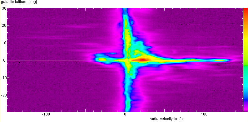
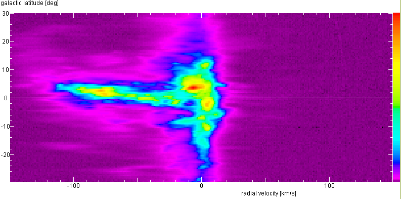
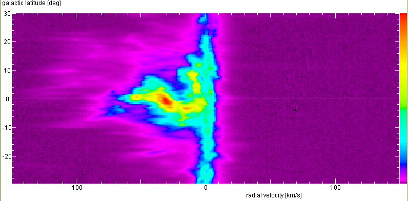
Below are the latitude-velocity maps from the original Leiden/Dwingeloo Survey data,
for l=20°
90°
150°
and 180°
The white horizontal line marks the Galactic Plane. Our plots cannot show structures as
fine or as faint as these, but the essential features will be there! What do they mean?
- in the Plane you find a large range of radial velocities.
- here, one also finds several maxima in intensity. These are the
various spiral arms
- there is a strong component at zero radial velocity: this is gas
in our neighbourhood which follows the Sun's motion in the Galaxy
closely: All around us is the gas from our own spiral arm.
- the anti-centre position (l=180°) does not show much variation in
radial speed, because the gas is essential on circular orbit about
the Galactic Centre, and in this direction we see all the motion
tangentially, hence with little radial velocity!
- at latitudes away from the Plane, the local gas still dominates,
but some gas at other velocities can be seen
| Top of the Page
| Back to the MainPage
| to my HomePage
|
last update: Feb. 2010 J.Köppen