Basic Radio Interferometer
Joachim Köppen DF3GJ ... Kiel, Aug 2016
Some brief explanations
- This is a simulation of a basic radio interferometer. It consists of of two (or three) antennas placed in a row at specifiable distances. All antennas are parabolic dishes of the same diameter and work at the specified frequency. There also is the choice of a single antenna, for comparison.
- The antenna pattern of a single dish is displayed by the green button antenna. One may choose between a sinc(x) = sin(x)/x and a Gaussian pattern. The Half Power Beam Width is computed from the wavelength and the antenna diameter.
- The Interferometer can be operated in two modes: either all antennas
are pointed to the zenith and the source passes over them (left) or
the antennas track the source while it crosses the sky (right). In
either mode the angle of the source is measured with respect to
the zenith.
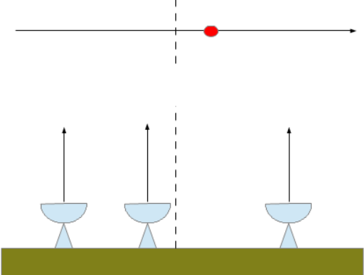

When the antennas are fixed on the zenith, the fringe pattern is modulated with the pattern of the individual antenna. - Several simple sky sources are available, with a specifiable angular diameter: top hat: the surface brightness is constant across the source, sun: source with limb darkening, triangle and a gaussian. A single 1-D source can be chosen, or a 2-D disc, as well as a pair of two sources, separated by a specified angle, and with a specified intensity ratio. The source surface brightness is displayed by the grey button source, and by a grey curve.
- How to use the simulator:
- Choose the antenna configuration:
- single dish, pointing at the zenith. The source passes through the zenith at angle=0.
- 2 or 3 dish adding interferometer. Both antennas point at the zenith, through across which the source passes.
- 2 or 3 dish adding interferometer. All antennas track the source.
- 2 or 3 dish correlation interferometer. Both antennas point at the zenith, through across which the source passes.
- 2 or 3 dish correlation interferometer. All antennas track the source.
- Choose the source, and enter all the necessary parameters.
- Click the red button result to show the red curve of the relative signal that would be measured when the source passes across the sky. Angle=0 denotes when the centre of the source passes through the antenna beam centre or the meridian.
- Choose the max.angle so that the main features are well displayed. If you choose too large a value, the displayed curve may show kinks or even look weird, because the curve's fine features are not well represented by the finite number of points.
- The ordinate - in relative power - can be displayed in linear or logarithmic manner.
- A click on one of the buttons source, antenna, result will choose the appropriate curve to be displayed. With clear one clears the plot and the choices, so that one may make other choices of what to display.
- The output button allows to display the numerical data of the results A and B at the bottom of this page. These are 400 lines of data. Simply grab the text with the mouse, copy and paste it into a text editor window for further use and storage as a simple text file. This may be imported or read by a program of your choice for further display and analysis.
- Visibility plot: while the data from a single antenna
gives a direct indication of the variation of surface brightness of a source,
interpreting interferometer data is neither direct nor easy:
- The output consists of fringes, whose angular spacing depends on the separation of the antennas (viz. the baseline), and whose amplitude contains the information about the angular size of the source.
- From the amplitude of the fringes one determines the visibility:
V = (ymax-ymin)/(ymax+ymin)
This is done by the simulation, and the value is displayed below the plot. - One measures the visibility for several baselines B.
Since the angular resolution of an interferometer increases with B:
FWHM = 58° / (B/λ) - which is given on the left hand panel - each observation yields information of how the source looks like at that particular resolution. - For the two and three interferometer with tracking the visibilities can
directly be plotted:
- click clear visibilities to bring up the plot and clear it
- enter another value for the 1-2 baseline, hit Enter key or click add a vis., and another datum is added.
- random 10 adds the results from ten random baselines. This is useful to get a first idea of the visibility curve.
- scan64 and scan512 computes the visibility curve with the indicated number of points. such a curve can be displayed in linear or logarithmic manner.
- note that the computation of a curve may take a bit of time.
- The numerical data can also be outputted by clicking output.
- If one were to try to get a complete coverage of the visibility curve with two antennas, this would be a tough and tedious job, setting them up at many baselines and collect observational data!
- Already with three antennas one obtains visibilities from the three baselines formed by each pair. Thus one observation gives three points of the visibility curve ...
- Since the projected baselines differ (like B sin(source elevation))
when seen from different sky positions, observing the same object on its
path across the sky yields visibilities from baselines that change with
time.
In this manner, one employs the Earth's rotation to give a more complete coverage of the visibility curve. - In a multi-antenna interferometer one may obtain complete coverage of the visibility (also in 2 dimensions), which permits to reconstruct the brightness distribution of a source (aperture synthesis).
- Interpretation of results:
- The aim of observations is to determine the dependence of visibility on the normalized baseline u = B/λ. This function (in 1D: visibility curve) is the (modulus) of the Fourier transform of the source brightness distribution. Thus from a good knowledge of the visibility function the source geometry can be reconstructed. Elementary cases are:
- The visibility of a pair of disk shaped sources is the visibility for a pair of point sources convolved with that for a tophat source.
- Summary: as long as the visibility is close to unity, the source is not resolved, and it needs a larger interferometer baseline. When the fringes disappear, a single source is fully resolved.
- For the convenience of faster computation, this simulation is done in one dimension: the sources are modelled only along the direction parallel to the interferometer, and they are assumed to pass over only in this direction.
- Also in the interest of fast results, the methods are chosen to give reliable results as long as the parameters are not too extreme ...
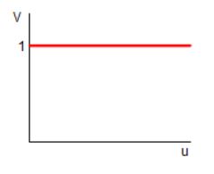 |
Point source always has V=1 for any baseline. |
 |
Gaussian source with a brightness profile like
exp(-a²/2σ²)
has V(u) = exp(-(2π u σ)²/2). This means that the visibility decreases for baselines larger than about λ/(2π σ), i.e. when the source is resolved. |
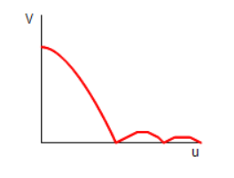 |
A source with uniform surface brightness and angular diameter d (in radians)
has the visibility V(u) = 2 J1(π d u)/(π d u) ("Airy disk" in 2 D) or V(u) = sin(π d u)/(π d u) in 1 D. Hence it will be small for antenna spacings larger than about λ/(π d) In particular, visibility becomes zero near u = 1/d |
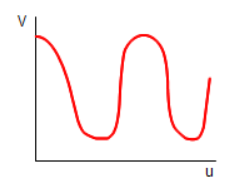 |
A pair of point sources with intensities A and B, spaced by an angle d (in radians): |V(u)|² = [(A-B)/(A+B)]² + 4AB cos²(π d u)/(A+B)² which varies between minimum and maximum values with a period 1/d in u. |
| Top of the Page | Java Applets Index | JavaScript Index | my HomePage |