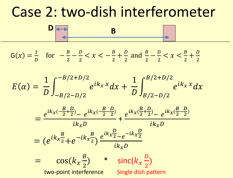
The outcome is simply the product of the pattern of a single antenna with a factor which describes the interference due to the distance between the antennas.
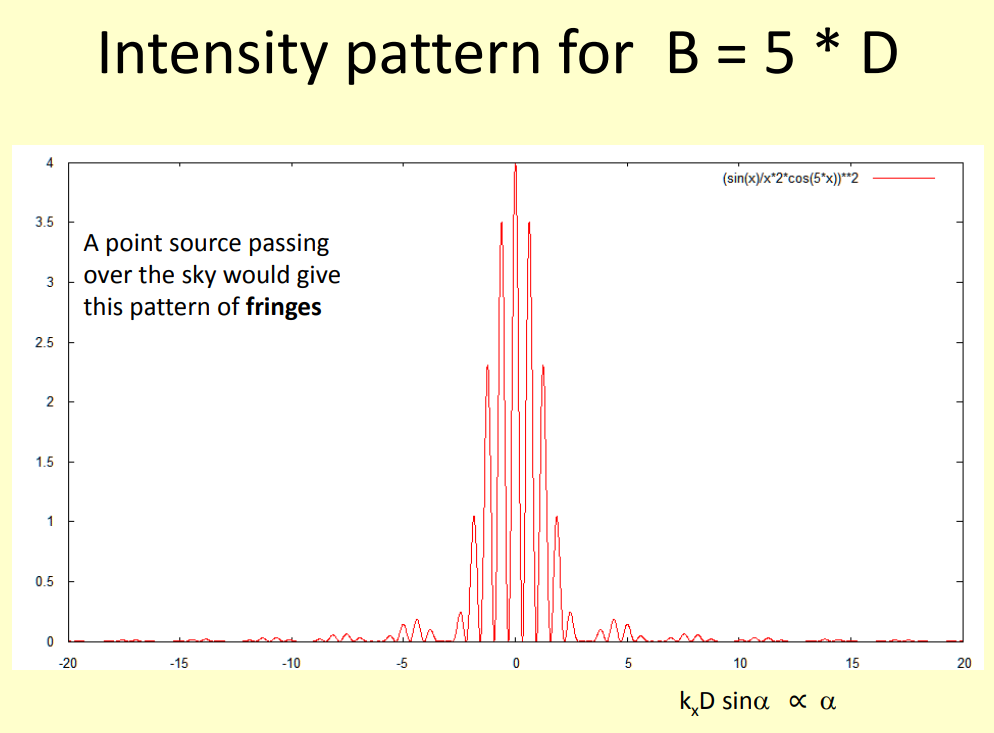
The radiation pattern - here shown as signal power - which is the sensitivity pattern on reception has narrowly spaced peaks - the interference "fringes" - whose angular separation is determined by the antenna separation B, but whose strength varies also more slowly depending on the antenna diameter D:
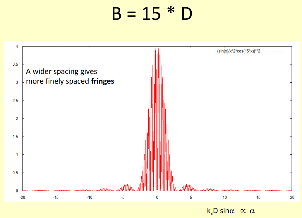
A greater baseline makes the fringes more narrow and also more narrowly spaced, but as the antenna diameter D remained the same, the envelope curve of the fringes remains the same:
This means that with two widely separated antennas one obtains a combined signal which offers a higher angular resolution than a single antenna, given by each narrow fringe. However, one pays with having to deal with a large and narrowly spaced fringes ...
... the remedy is to use more antennas, and placing them at suitably chosen separations, to concentrate the radiation pattern into fewer and more widely separated fringes ...
Let us return to the two-antenna interferometer: Let us first consider the radiation that arrives from a point in the source - the angle θ is the angle between this direction and the direction perpendicular to the baseline b (the dashed vertical line).
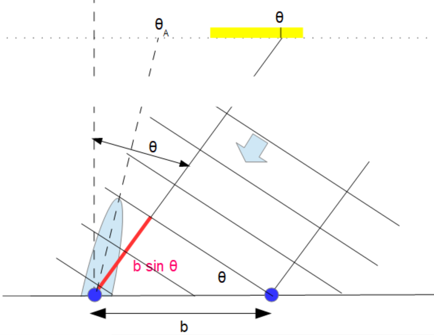
The time delay of the wavefront arriving first at the antenna on the right and later at the one at left gives rise to a phase difference of
φ = kb sin(θ) = 2π b/λ sin(θ)
between the output voltages of the antennas (with the wavenumber k = 2π/λ):
U1 = U0 cos(ωt + φ/2) and U2 = U0 cos(ωt - φ/2)
In the adding interferometer the two voltages are added at the receiver input. The amplitude of the sum signal is its time average:
< U1 + U2 > = 2 U0 cos(φ/2)
and the received power is
P = < U1 + U2 >² = 2 U0² (1 + cos(φ))
As in optical interferometry one measures the maximum and minimum of the fringes, and calculates the visibility
V = (pmax - pmin) / (pmax+pmin)
When a source is unresolved by the instrument, the fringes are large and V = 1; a fully resolved source shows no fringes, hence V = 0.
This type of interferometer was used in the early years of radio astronomy, from 1945 to the early 1950. But soon it was realized that by phase-switching (M.Ryle, 1952, Proc.Roy.Soc.A 211, 351) or continuous multiplication of the signals (E.J.Blum, 1959, Annales d'Astrophys. 22, 140) interferometers can be operated in a better and more efficient way, as one looks at the correlation between the signals from different antennas. This is now the way all interferometers work.
In the correlation interferometer the signals from the two antennas are multipied with each other and and time-averaged. For easier manipulations we write this in complex form:
U1 = U0 exp(-jωt + jφ/2) and U2 = U0 exp(-jωt - jφ/2)
This gives as an instrument response:
R = < U1 * U*2 > = U0²< exp(-jωt + jφ/2) * exp(jωt + jφ/2) > = U0²exp(jφ) = U0²(cos(φ) + j sin(φ))
The correlator thus provides two outputs: the real (cosine) and the imaginary (sine) parts of the visibility. It is convenient to record these as visibility magnitude and phase; often the magnitude is called the visibility amplitude.
Now let us consider this in some greater detail: Suppose the antennas point at angle θA which might differ from the centre of the source θS. If we integrate the instrument response R(θ) from the point θ in the source:
R = ∫ A(θ-θA) S(θ) exp(j φ) dθ
Here, A(θ-θA) is the sensitivity of the antennas which point in direction θA, and S(θ) is the brightness of the source at position θ. With a fixed antenna pointing (constant θA) the source is observed while drifting through the antenna beam. When the source is tracked, θA = θS. The phase angle is:
φ = 2π b/λ sin(θ) = 2π u sin(θ)
If we define the spatial frequency u = b/λ we recognize in:
R(u) = ∫ A(θ...) S(θ) exp(j 2π u sin(θ)) dθ = ∫ A(θ...) S(θ) exp(j 2π²/180° u θ) dθ
(especially for small angles θ) that the instrument's response is the Fourier transformation of the product A*S. For the ideal case of isotropic antennas or the realistic case of using antennas whose radiation pattern is wider than the source size the inverse Fourier transformation of the instrumental response R(u) - viz. the visibility V(u) - gives the brightness distribution of the source.
Hence, the measurement of the visibility function, i.e. its dependence of the spatial frequency u allows us to reconstruct the image of a source.
| Top of the Page | Interferometer Explorer | JavaScript Index | my HomePage |