The Hydro Applet is the simulation of the movement of gas in a linear tube. It shows the evolution of the density, velocity, and temperature of the gas, starting from an initial situation which the user can specify.

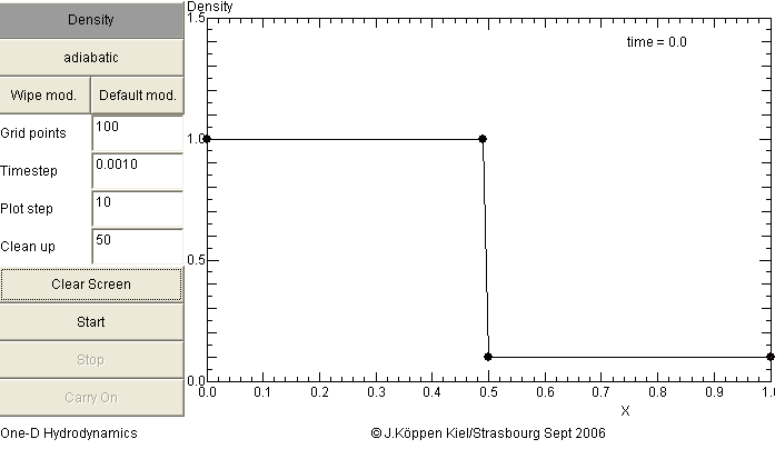
The applet starts with the default model which is a rather simple but fundamental example: In the beginning, the left half is filled with gas of high density (value = 1), while the right half is partial vacuum (gas density at a lower value of 0.1), separated by a thin membrane. In both parts, the gas is at rest, i.e. there is no systematic flow in either direction. At time zero, this membrane is suddenly removed, and the gas rushes from the left side to fill the vacuum. This happens with some interesting features, which can be nicely seen in this simulation. The linear tube is a classical example to show the formation of shocks in hydro- and aerodynamical flows. When you click Clear Screen you get this view of the initial density profile:

The left hand panel allows the user to operate the simulation and specify some parameters and options:

• the dark gray Button Density navigates to show Velocity, Temperature, and all together quantities
• the Button adiabatic indicates this treatment of the energy equation. Clicking it, changes over to the isothermal case which assumes a temperature of 1.0
• Wipe mod. clears all data points of the initial profile for the shown quantity: density, velocity, or temperature. The other remain unchanged. To make another model, you have to specify these initial profiles in all three quantities (or two in the isothermal case). To enter new data, you simply click with the mouse pointer on the area of the corresponding graph. The entered data is shown as dots; you can modify the profile by dragging a dot to a different position. Between the dots, the simulation will interpolate linearly. Note that you can enter or modify data only on the plots that show only one quantity!
• Default mod. puts in the simple shock tube
• Grid points specifies the number of points of the spatial grid (maximum is 1000). The more points you have, the better is the resolution, but the time step has to be made smaller ...
• Timestep is the time intervall between two successive models. The smaller the better! But if you chose too large a time step, the applet will impose the Courant-Friedrichs-Levy condition. This is the largest time step one can apply before the calculation gets unstable.
• Plot step is the number of time steps after which a new curve is displayed. Entering 1 means that every time step is shown ... which might fill the screen with curves too densly spaced
• Clean up to prevent the plot to become cluttered up with curves, the screen is cleared after ... curves. A value of 1 will display only one curve, the situation at that moment
• Clear Screen, Start, Stop, and Carry On are the Buttons to control the simulation. If you display the density, but want to see what happens with the velocity, you can either display all together or swapping between plots by this trick: Stop the simulation; now you can look at all the curves for the current moment by clicking the navigation button (top left); and then you may Carry On with the run.

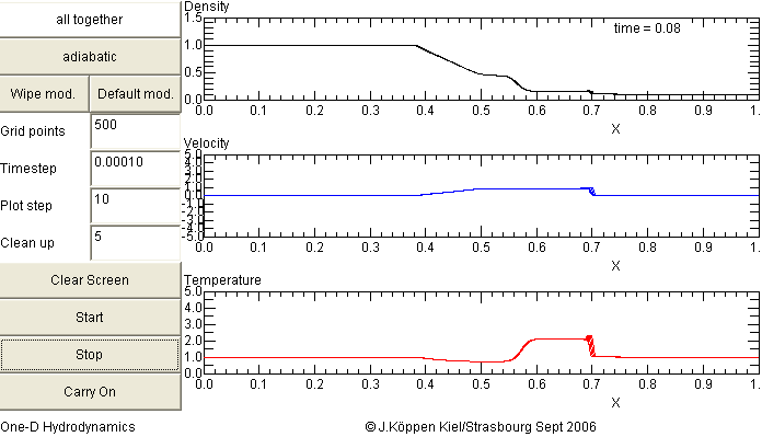
Here is the result of the simple shock tube - in the adiabatic case - which we stopped at 0.08 time units

In the velocity plot, one sees the flow speed of the gas to the right (positive velocity) and to the left (negative velocity). The gas in the left hand half starts to move slowly to the right, at the position where the partition had been, the speed reaches 1.0, it stays constant right up to the shock (at position 0.7) which marks the extreme position up to which gas has penetrated the empty region. The density profile shows the rarefraction wave - where the gas moves with increasingly greater speed - the contact discontinuity - at position 0.56 - and the shock as two jumps in density. In truth, these jumps are discontinuities, but in the numerical solution there are somewhat smeared out, because it is difficult for our simple method to treat accurately any sharp jumps in the solution. The temperature profile shows that the gas between shock and contact discontinuity has been heated up.

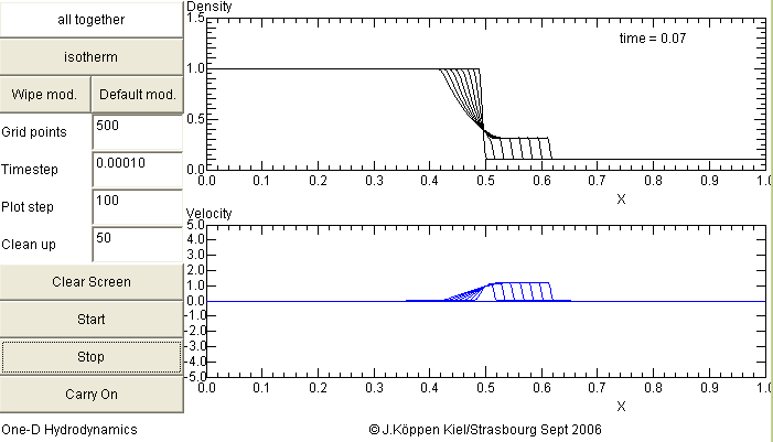
The shock tube in the isothermal case - the temperature is set to 1.0 - looks similar: There is the shock and the rarefraction wave, but the contact discontinuity is absent.

Some experiments:

• with the density contrast of 0.1 as before, isothermal models even with 20 points, a time step of 0.01 and making 1000 time steps between plots gives a nice impression of the overall happenings.
• the treatment of the reflection of the gas waves with the right and left boundaries of the tube is rather simple and not very accurate. The waves produced by such a reflection are not to be taken as reality ... if you run the isothermal simulation for a long time, the density profile will finally settle into a nearly constant value. You will notice that the density is not exactly 0.5 as mass conservation demands, but also that the waves that go back and forth diminish in amplitude. This means that the code loses some of the energy ... it would be too much to ask from a simple method be able to match reality precisely!
• with more space points and sufficiently small time step, increase the density constrast. Observe the speed of the shock
• with high contrasts (low density snaller than about 0.01) it is wise to start the simulation with very small times steps, stop it, increase the time step, and carry on the simulation. This can be done several times, increasing the time step progressively.
• a large number of space points and too large a time step usually gives rise to waves in the region behind the shock, which become bigger and bigger, until a negative density or temperature stops the model.

About the units: We use normalized units:

• the length unit is the length of the tube
• the time unit is the time in which a sound wave (at unit temperature) crosses the tube once
• the velocities are measured in sound speeds
• the temperatures are given as the square root of the sound speed; in other words: the sound speed at unit temperature is also unity
• the density is completely arbiratry, since the solutions for this simple problem doe not depend on the actual values of mass or density

About the method:

The model is described by a system of two (or three) partial differential equations, the conservations of mass and momentum (and energy). This system is formulated in a conservative way, by considering how the mass and momentum (and energy) of each parcel of gas are changed by the interaction with the neighbouring parcels. A simple explicit method is used to compute the time evolution.