Solar Eclipse 2015

|
The total solar eclipse on 20 march 2015 had the greatest eclipse in Kiel at 09:46 UT
and the Sun was covered by about 80 percent. First contact occurred at 08:38 and last
contact at 10:56 UT ...
|
|
... but as the high fog arrived right on time, we at
DL0SHF, the Radio Observatory and Ground Station in Rönne
did not see anything.
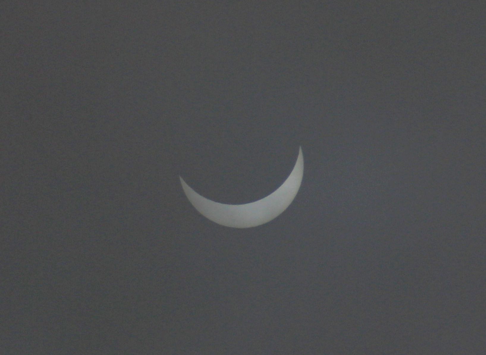
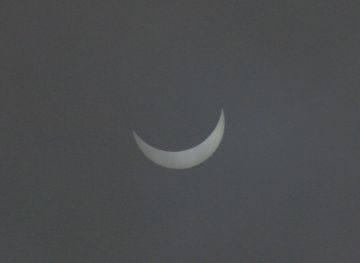
Fortunately, Hermann Fenger at our 'outstation' in Bielefeld enjoyed a glimps through
the clouds and took the visual image at 10:54 UT. Focal length 200 mm, exposure 1/320 s
at ISO 100 and f-stop 7.
|
|
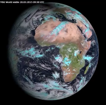
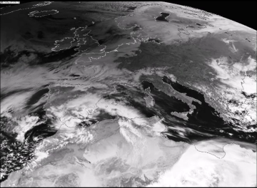
From the images in visual light by Meteosat received at DL0SHF two
movies were compiled: the one on the left shows the entire Earth disk in colour
during the entire day. The one on the right shows in greyscale how the penumbra
passed over Europe. Click on the image to start the video.
In these images the umbra is too small to be visible, but the penumbra of a few
thousand km size.
The original images have 768 by 576 pixels. The registration of a single image takes
about 12 min, since every image is read line-by-line. The images, taken
every 15 min, are sequenced together in Rönne to form the video.
|
|
|
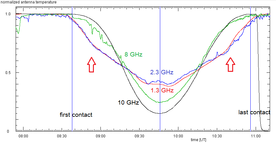
At DL0SHF, we observed entire eclipse on 1.3, 2.3, 8.2, and 10 GHz. The composite plot
shows the evolution of the antenna temperatures, normalized to the value before the
eclipse. This linear quantity presents the fraction of the solar flux received on each
frequency. One notes:
- at maximum eclipse the signal is lower the higher is the frequency. This is because
at higher frequencies the radiation comes from deeper layers, close to the visual
'surface' of the Sun, the photosphere. At low frequencies the emission comes from
the corona which extends well above the solar 'surface'.
- at low frequency the signal starts dropping before it drops at high frequency, and
before the first contact in the optical. At frequencies below about 3 GHz the emission
comes from the corona, which is the zone of very hot gas which extends above the
photosphere and up to a few solar radii. The Moon covers parts of this region before
it touches the solar disk.
- at 10 GHz the curve is shaped like a 'V' while at 1.3 GHz it resembles a 'U'
- at 1.3 and 2.3 GHz the curve has slight kinks (red arrow points at the one after
maximum eclipse) where its slope changes somewhat ...
- also at 1.3 and 2.3 GHz, there are two small dips in the signal near maximum
eclipse. That they appear at both frequencies proves that this is not an instrumental
effect or defect. Could it be due to a change in the Earth atmosphere, like passing
clouds?
|

|
Here are the explanations: In the optical and also at 10 GHz the Sun resembles
a disk of nearly uniform brightness. In a simple model for the eclipse one
obtains a 'V' shaped profile of the flux fraction. In this model the Moon passes
in horizontal direction over the Sun. The distance between the centres of their
disk is set to give a maximum covering of 80 percent, as it is predicted for Kiel.
The signal drops right at the moment of first optical contact, of course!
|
Here is the RadioEclipse interactive simulator
|
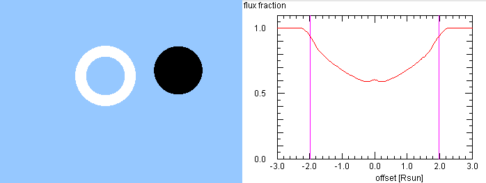
On 1.3 and 2.3 GHz the radio emission comes from the corona, which lies above
the photosphere. If we model this with a bright ring, with inner radius 0.8 and
outer radius 1.25 (in radii of the optical solar disk) we get:
- the curve has a shape like a 'U'
- the signal starts dropping before the first contact (marked by vertical
magenta line)
- at offsets of -1.5 and 1.5 solar disk radii the slope of the curve changes
slightly but markedly. This is due to the way the Moon covers the emission
ring, which is slightly larger than the Moon
- at maximum eclipse, there is a slight peak in the signal. This is because
the Moon can only cover the inner parts of the coronal emission, but not
the outer rim
- before and after this peak there are slight depressions, just as they are observed
on 1.3 and 2.3 GHz. Therefore these dips are not passing clouds, but the
consequence of the Moon covering a brighter spot at the Eastern side of
the coronal emission.
|
Here is the detailed Report on Observations, Data Reduction, and first Interpretation ...
... and here: Report on the Modeling of the Observations
|

|
|
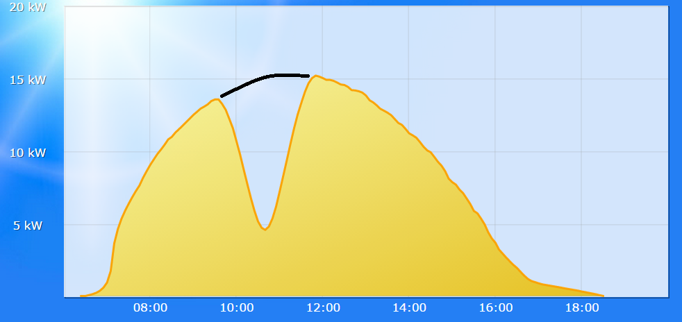
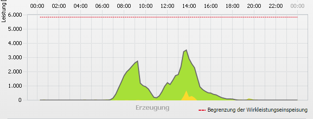
Despite the grey skies in Northern Germany, records from a solar photovoltaic system
give solid proof that it did occur here, too ... ;-)
|
A record from Southern Germany allows to deduce the mininum fraction of light to be
31 percent, which agrees well with the 30 percent predicted for this place.
|
Some Background on the Radio Sun:
Radio emission from the Sun is the long-wave extension of its thermal radiation
in the optical and infrared ranges, which is produced by the warm and hot plasma.
Apart from a constant 'quiet' component there appears also in times of high activity
short or long periods of enhanced radio emission. These are caused by regions of
enhanced temperature in higher layers and expelled plasma clouds (CME 'Coronal Mass Ejections').
The layer which from optical observations we could call the surface, is the photosphere
with a temperature of about 6000 K. This is the deepest layer accesible to direct observation,
since here the density increases strongly with depth, and thus the increasing absorption
blocks the view. Above the photosphere, the temerature continues to decrease, to about
4300 K, and then increases again towards the chromosphere, which is only prominent
during total solar eclipses due to its emission lines. Above the chromosphere there is
the Transition Layer, in which the temperature increases from about 10000 K to
several hundred thousand K. Above this extend the Corona up to several solar radii,
with very low density and temperatures of millions K.
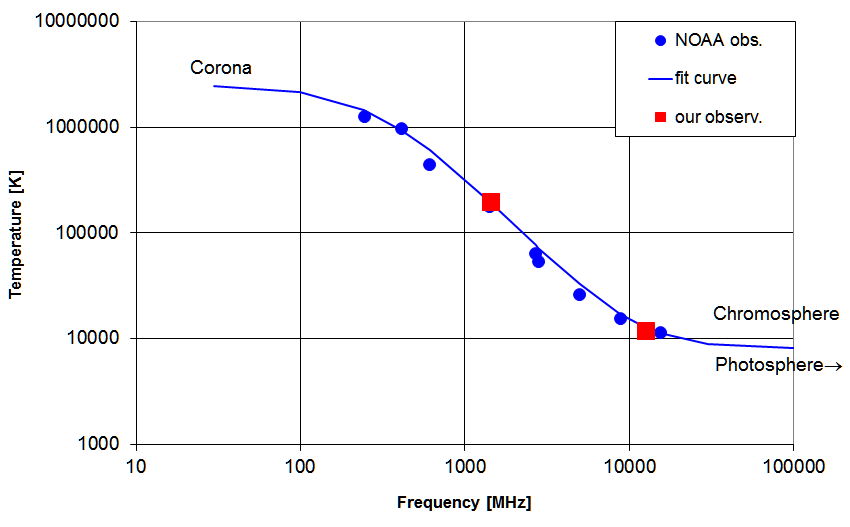
Since the absorption of the solar plasma incleases towards longer wavelengths, it
is not possible in the radio range to look as deep as with visible light. The radiation
originates from higher layers the lower is the frequency. At 10 GHz one reaches already
only down to the upper chromosphere, below 1 GHz the radiation comes from the Corona. In
this way radio observations at different frequencies allow to probe the temperatures
in the various layers of the solar atmosphere. Solar radio fluxes are measured several
times each day by an international network of radio observatories, and the data are
published almost real-time by NOAA.
The spectral distribution of the radio fluxes
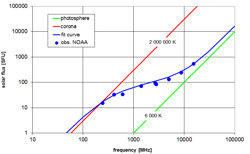
maps the temperature stratification in the solar atmosphere:
Determination the Solar Radio Flux
Four measurements are required:
- direct signal from the Sun: p(sun)
- sky background at the same elevation: psky(ε)
- flux calibration: pcal
- antenna half-power beam width: HPBW
All measurements can conveniently obtained by a drift scan:
- point antenna to where the Sun will be in about 10 min
- continuing recording of data will show the noise increase when the Sun enters
the antenna beam ...
- ... passes through a maximum (this gives p(sun)) ...
- ... and decreases again
- after this (or best also before!) the antenna is slewed at constant elevation
to a position far enough from the Sun, so that no solar radiation is picked up
through the side lobes. At this elevation ε the sky background is
measured: psky(ε)
- after this (or best also before!) one does a flux calibration:
pcal
This may look like this observation on 1.3 GHz. The ample time before and after
the passage of the Sun allows also to pick up the antenna's weak side lobes.
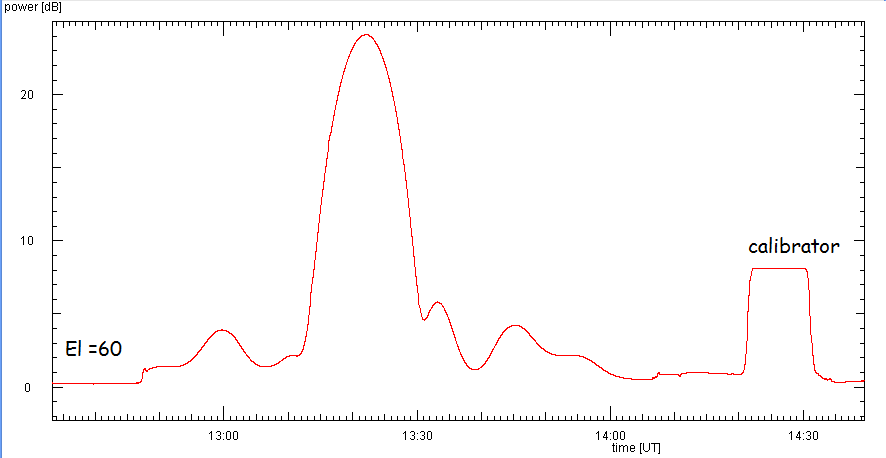
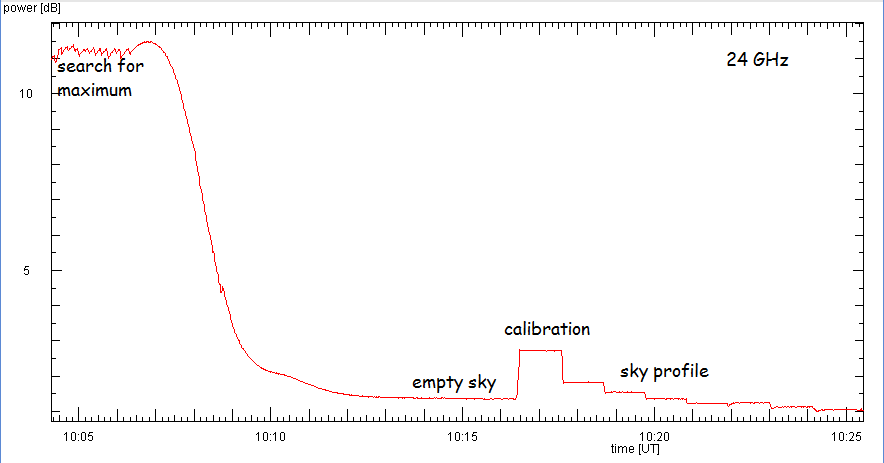
This procedure requires an accurate pointing system. If this is not available, one
can first search manually for the maximum signal from the Sun, then with the fixed
antenna watch the Sun on its way out of the main lobe. Such a half-scan also yields
all necessary information and takes less time:
Interpretation
One follows this procedure: In the fundamental relations for the solar signal (in linear power)
p(sun) = a (Tant(sun) + Tzenit/sinε + Tsys + TCMB)
and for the sky background
psky(ε) = a (Tzenit/sinε + Tsys + TCMB)
one determines the unknown scaling factor a from the flux calibration:
pcal = a (Tcal + Tsys)
- Using the measured sky background value directly, the knowledge of the system temperature
suffices to derive the antenna temperature of the sun:
Tant(sun) = (Tcal + Tsys)*(p(sun) - psky)/ pcal
- If one knows from the analysis of the
sky background both system and zenith temperatures - or due to the good stability
of the system one may assume their validity - one may use this form:
Tant(sun) = (Tcal + Tsys)*p(sun)/pcal
- (Tzenith/sinε + Tsys + TCMB)
- Since on 1 GHz the zenith temperature appears to be pretty constant, one may also
derive the system temperature:
Tsys = (psky(ε) Tcal - pcal(Tzenit/sinε + TCMB)
/(pcal - psky(ε))
Radio Flux
With the knowledge of the effective area Aeff of the antenne the radio
flux (in Jansky) is obtained:
Fsun = Aeff/2760 * Tant(sun)
Solar Surface Temperature
The derived antenna temperature is not yet a direct measure of the physical temperatur
on the Sun, since it depends on the properties of the antenna:
- if the solar disk with its angular diameter of about D = 0.5ş is smaller than the
antenna beam width (i.e. HPBW) - as it is with the 1.3 GHz and 2.3 GHz dishes -
the true temperatur on the solar surface is higher via the beam filling factor:
Tsun = 1.5393 * Tant(sun) * (HPBW/D)2
The first factor is a correction for the shape of the antenna beam.
- only if the Sun fills completely the antenna lobe - as with the 10 GHz and 24 GHz dishes -
antenna and true temperatures are the same:
Tsun = Tant(sun)
Half-Power Beam Width
Thus the knowledge of the antenna's beam width is required. As this is an unchanged
property of the hardware, a single measurement suffices. It comes free as a by-product
of a drift scan: the HPBW (Half-Power Beam Width) is defined as the full width of the
antenna's main lobe at half the maximum power. Since in a drift scan the accurate rotation
of the Earth provides the horizontal movement of the Sun, one measures the time interval
during which the measured (linear) power (above the background) exceeds one half of the
maximum. In one hour the Sun at its present declination δsun moves over
an angle of 15ş cos δsun.
Another method is to match the data (red) by a Gaussian profile (blue), as shown below.
Here one also notes how well the antenna characteristic resembles a Gaussian function
and where it differs. The green line is the level at half maximum power. The black
arrows indicate up to where measurements for the main lobe should reach.

| Top of the Page
| back to my Home Page
|