About error bars

About Error Bars

Joachim Köppen Strasbourg 2008

With any measurement we have to be aware that all our data and hence all our results are not infinitely accurate, and we have to think about errors: their type, their sources, and how to estimate them. Unless we do this, we cannot be sure that our results are reliable or useful!

The types of errors are:

random errors: are due to the random noise which affects the data. our case the data are in fact noise from e.g. the sun, but whose amplitude will show fluctuations. Part of the fluctuations will be due to the noise generated in the receiver, and which thus will affect all measurements: of the source, of the flux calibrator, and of the (sky) background!
discretization errors: in the measurement receiver the analogue voltages from the detector is converted into digital form before passed to the computer. The resolution of this conversion is 0.1 dB. Thus a datum of +43.3 dBµV may mean anything between +43.26 and +43.35 dBµV. If the real datum is +43.35 dBµV, the output would be hopping between +43.3 and +43.4, with about equal probability.
systematic errors: since we do not measure ourselves and every day the temperature of the walls of the Holiday Inn, there will be an uncertainty on the temperature of our flux calibrator. For simplicity, we shall assume that its does not vary much from day to day ... but it is obvious that observations in summer might be different than in winter ... so far, we have not taken that into account, and simply assumed a constant value of 290 or 300 K. There could also be other factors, for instance whether our value of the HPBW is OK, which we used for correcting for the beam filling factor. Likewise the antenna pattern may have sidelobes through which unwanted radiation enters. Such an error would result in giving numbers always a bit too low or too high. Finally the sky's contribution to the background noise we have so far neglected, thus our results might be different for different elevations ...

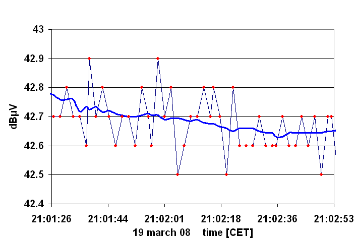
Let us consider random errors: Here is an example of measurement of the sky, on a relatively clear night:

The raw data consist of a series of points, which obviously fluctuates randomly about some average level. [The discerning eagle eye will notice that there is a certain downward trend in the data - but whether this is real or meaningful or interesting, is a different matter ...] First of all, this stretch of data would constitute a measurement of the background. But how to get that value?

If one were to take only one measurement, it is obvious that one would be in danger to pick anything between a value too low up to a value too high.

Therefore we observe always a stretch of data, that is sufficiently long so that we can extract a meaningful average value: in the example, one would obtain a mean value of +42.69 dBµV ... or should one take +42.6941477328... as it is displayed by your software? Who would be so silly to take seriously all these decimal places?

But how many decimal places can one trust? In other words: what is the error bar? We can simply compute the variance or dispersion of the data points around the average value: the r.m.s deviation from the average! This comes out as 0.11 dB in our data. Thus we can say that the background value is

+42.69 +/- 0.11 dBµV In other words, the second decimal place is not reliable, and we really mean +42.7 +/- 0.1 dBµV and this is really what we should write and publish and accept! Further decimal places are meaningless - however, sometimes we give one decimal place more than necessary, in order to prevent rounding errors if someone uses our value for something further.

We also see that the raw data comes only in discrete steps of 0.1 dB. This is the resolution of the analog-to-digital converter of the receiver. A value of 43.5 can mean anything between 43.45 to 43.54! Thus, we have a discretization or digitalization error of +0.05 dB for a single measurement. If one considers a sufficiently long stretch of data, one can hope that this error cancels out on the average. So we do not need to consider this further ... however, the data set must be sufficiently long, and in principle we should keep that in mind.

In the computation of the average and the dispersion we assume that the measurements are to be represented by a constant single value plus some random noise. If our data set is rather long, often we may also apply a smoothing algorithm to the raw data. Hereby we substitude the value of one point by the average taken over a number of points in the neighbourhood. Evidently, the more points we have to smooth over, the less bumpy will be the resulting curve, and if there are any interesting structures, we might not want to wash them out. Such a smoothed curve will still show fluctuations: In our example, we averaged over a neighbourhood of twenty points (ten places to the left and ten places to the right). If we now take the average, we get the same number as before, but the dispersion is much lower: 0.03 dB. This is because we have used at every point more information than before. If we now want to describe the raw data with the smoothed curve, we can say that the uncertainty of placing that curve where it is, is +/- 0.03 dB.

Obviously, the longer is the data set, the longer we may make the averaging, and eventually we average over the entire data set, and get a very low dispersion. If one does a proper mathematical analysis, one obtains the following expressions for the analysis of the data values: x_1, x_2, ..., x_n

the average value is <x> = (x_1 + x_2 + ... + x_n) / n
the dispersion is s² = ((x_1-<x>)² + (x_2-<x>)² + ... + (x_n-<x>)²) / n
the error bar for the average is +/- s / sqrt(n)
the error bar for the dispersion is +/- s / sqrt(2n)

This means that for the interpretation of solar observations we have to consider and determine (or estimate) three random errors:

on the solar signal - i.e. one fits a curve through the data and determines the peak value
on the backgound signal
on the calibrator signal

In the final result, all three errors will add up ... but since they are random errors which we can assume to be independent of each other, hence the error bars sum up quadratically: s²_total = s²_signal + s²_calibration + s²_background For example: from a stretch of about 50 data points (as shown above) we get from the averaging of the raw data an error bar of about 0.1 dB/sqrt(50) = 0.014 dB for each of the three measurements. Thus, the total error bar will be 1.732 * 0.014 dB, or about 0.024 dB which is about 0.56 percent relative error (in linear terms). Therefore, our uncertainty on the derived (solar) temperature of 10000 K will be +/-60 K.

On top of this will come any other random errors and of course any systematic errors ... if we use a calibrator temperature and thus neglect a possible variation between 0 to 10°C, we have another uncertainty of up to 3 percent, which is much more than the random errors! The resultant total error would then be 300 K for the solar temperature ... This example shows that one has to carefully consider the various sources of errors!

This final error bar will be the measure of whether deviations are large enough to be called significant, or otherwise be regarded only as chance fluctuations.

... and if your data agrees with the predictions by less than that error bar, you can be happy ... and if you data disagrees with predictions or theory by more than the error bar, you could also be happy, because you might have discovered something ...

As we had noted, there also is a tendency in this data set ... The way to extract that is called "Linear Regression" which means that we search a straight line whose parameters (slope and intercept) give a best fit to the data, in the sense that the r.m.s. deviations of the data points from the line are minimized. It goes beyond these pages to explain that ... but you find this described in standard textbooks of maths, statistics, or those which deal with methods of interpreting data.

But what if the data suggests not a straight line but some curve? Again we can formulate an optimization problem by trying to find that curve which gives the best match ... Obviously this is something more complicated, and you have to refer to maths and numerics literature or cook your own method.

| Top of the Page | Back to the MainPage | to my HomePage |

last update: Apr. 2013 J.Köppen