Basics
If we want to use the telescope data for quantitative measurements of the Sun, satellites and the Moon, we need to calibrate it in terms of the radio flux that enters the telescope. The numbers we get from the receiver are only a relative measure (in dB over 1 microVolt), and they pertain to the input of the receiver only. Thus anything that happens in the cable, in the LNB, and in the parabolic dish, we don't know ...
The designers supplied us with their Flux calibration report.
However, the properties of the receiving system change not only over time, but also vary from day to day, and even during a longer observation. Thus we need to flux-calibrate the instrument before and after a measurement, by comparing its output with the signals measured of a radio source of known properties. A convenient way is to use the thermal radio emission of the ground - or a nearby building, like the Hotel - its temperature will be close to 300 K, or if we want to be more accurate or conscientious: between 273 K (for 0 deg C in winter) and 333 K (for 30 deg C in summer)! When we point the telescope to this building, the entire antenna beam is filled with this radiation, and therefore corresponds to this known temperature.
The power measured by the receiving system of a radio telescope is basically noise. It is the sum of various components: usually the internal noise of the electronics (in particular of the first transistor in the LNB) gives the major portion, while the radiation from the astronomical sources constitute only a small portion. There also is the noise from the thermal radiation of the Earth atmosphere, thermal ground radiation reaching the LNB feed horn from the sides. Finally, noise from electrical machines and electronic gadgets (computers, computer displays, switched-mode power supplies) can make life difficult...
The received power is just the sum of all this! The objective of the flux calibration is to measure the noise level that a telescope receives in the absence of an external source. The system temperature is the temperature which gives the same noise power (Note that because the power of thermal noise is proportional to temperature: p=kBT, with Boltzmann's constant kB, temperature is a convenient measure of power!)
Primitive Version
Let us first consider a crude but simple method of flux calibration: We shall assume that only the internal noise from the receiver is important and that the sky is perfectly cold.
- point the telescope to the calibrating source. Make sure that the source fills the entire antenna beam. The received power shall be named p(cal). Note that this is the linear power, not the deciBel value!
- then point to the empty sky - some point conveniently high in the sky (perhaps 60° elevation) as we should avoid the horizon with trees and buildings. Call this power p(sky).
The first measurement gives:
as the received noise is the sum from the calibrator and the internal noise. The factor a is an unknown scale factor, which we need to determine.
The second measurement gives:
as we had neglected the noise from the sky. In principle, we could have assumed the 2.7 K from the cosmic microwave background ...
From only two measurements we can determine the system temperature
as well as the scale factor
Full Method of Flux Calibration
However, this simple method neglects the atmospheric noise, which is important at 11 GHz, and whose neglect could lead to systematic errors in the data deduced from the observations. A better method requires more measurements and a somewhat more complex interpretation.
While the internal receiver noise and the 2.7 K Cosmic Microwave Background (CMB) are the same for all elevations, the sky noise varies with elevation. It increases towards lower elevation. Fortunately this variation can be easily modeled, because the noise comes from the troposphere, which is only a very thin (8 km) layer of the Earth atmosphere. It thus can be treated as a plane-parallel layer, and the noise power is proportional to 1/sin(elevation):
where Tzen is the temperature extrapolated to the zenith.
Thus, measurements of the sky noise at several elevations allow us to separate the
sky noise from the other components, as shown in a schematic plot
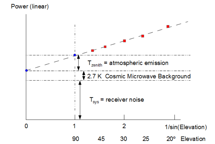
Red squares represent measured data, the blue dots mark points that are extrapolated from
the data.
The interpretation is straight forward: Matching the data with a straight line results in the line slope m and the Y-axis offset b, the value at 1/sin ε=0. This value is not represented by any real elevation angle, but one would obtain this extrapolated value in the absence of the Earth atmosphere!
The data are a measure of the power received by the antenna, but expressed in some arbitrary units, determined by the apparatus. If these are given in dB (deciBel), they need to be converted in linear powers (p = 10dB/10). In order to convert the raw values into antenna temperatures, we need to determine the scale factor a:
which includes all contributions from the source, the atmosphere, the receiver, and the microwave background. To resolve this, we execute a flux calibration: the antenna is pointed to the ground, a building, or a nearby dense grove of trees, which fills the antenna beam completely with its thermal radiation (at Tcal = 290 K):
Since we do not point to the sky, there are no contributions from atmosphere and CMB. From the sketch one recognizes that
Hence the scale factor is