Contents
This tool was written to permit the easy interactive handling, selection and visualization of the data of a relatively small number of objects - the present version is suitable for about 5000 objects and up to 100 properties. Applying it for more data will make loading and transfer times painfully long, and will of course also slow down all operations such as plotting. Also, depending on your browser (and its version) the display of too many properties by the Choice buttons may not be possible (e.g. in Netscape 4.7 you'll get one long list which does not fold to show all items). But that is dependent of how the Java elements are interpreted by the browser on your machine. This is a Java applet, which means that it runs on the machine of the user and is independent of the operating system of that machine.
Since I am still working on improvements, some of the screen shots have changed a bit .....
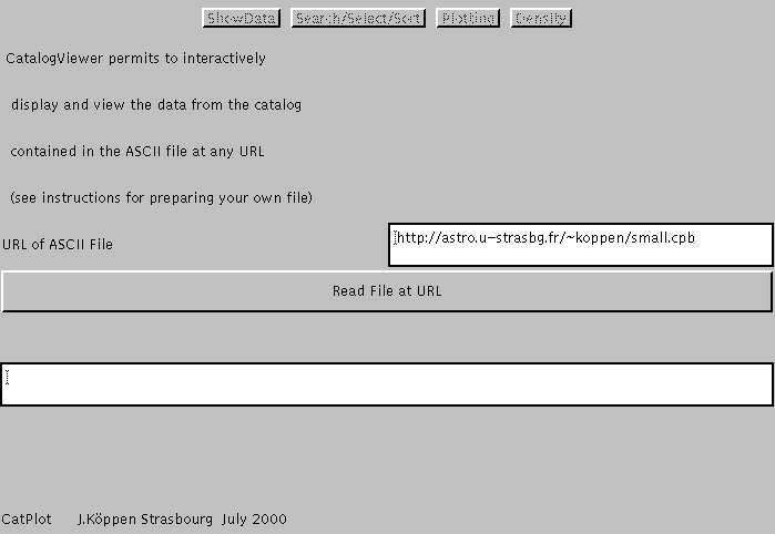
The first page -- which appears only once, at the beginning -- requests to enter the URL of the catalog file. Clicking the button reads in the file, whose number of objects and columns are then displayed in the text window, and the control buttons are enabled.

The current test version shows up with this
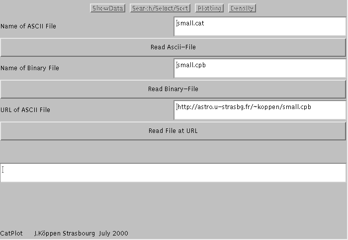
And after one has clicked read ascii file one gets the message that the catalog has been constructed
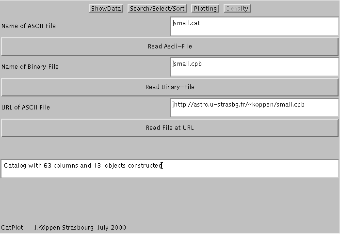
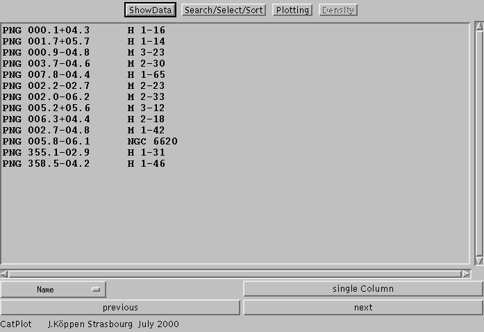
Note The current version is really designed to read once one catalog. This is why you'll never get back to this page once you've left it, and why all read-buttons are disabled after reading a file. However, there will be a version which allows to switch to another catalog when you're done with the first one. Clicking the ShowData button brings up the page which displays the data of the objects as a text table. One may look at one single column for a chunk of 20 objects:
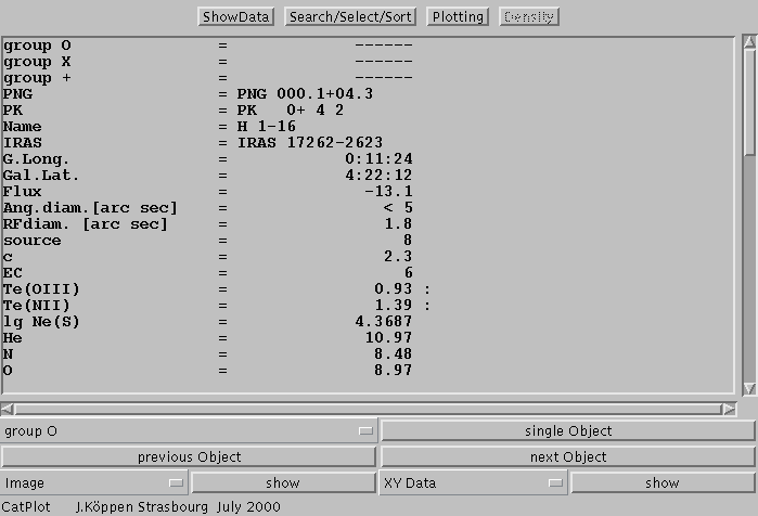
The first three entries in the data table, marked group O, group X, and group +, refer to the three groups of objects which can be selected interactively in the Plot (see below)............... If the object would have been selected in this manner, it would show up with a "yes".
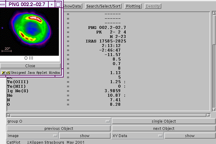
If one is in the mode where single object are shown, one can also view images and x-y plots that may exist for an object: The Choices permit to select with king of images or plots (if the catalog contains several ones). The neighbouring show button makes the data visible. If there is no data for an object, the button is disabled. If there is an image, a new window will open, as partially shown here - with a test image, not of M 2-23, but of the Ring nebula (grabbed from the Tübingen Image Gallery ). The size of the window can be modified by the user to suit his needs.
If one has called up a x-y plot, also a new window will open, showing the plot. With the controls Drag & Zoom one can use the mouse to zoom in any part of the plot. unZoom will restore the full view. The x and the y-data can be shown in linear or logarithmic fashion, using the relevant buttons linear X. If the data contains negative numbers, the logarithmic plot will usually represent them by values below what is shown.
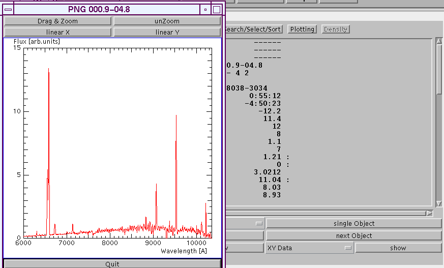
To close each window, click the quit button.
The control button Search/Sort/Select changes over to this page:
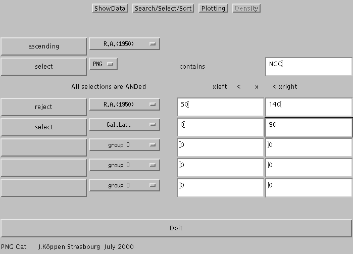
Then one can select all objects in whose text of the chosen string column (here: PNG) a certain string (here: NGC) is found. This selection is case sensitive and does not ignore any blanks, so the search string must be typed in as it really is. Clicking the button switches between no-action, select, and reject.
Furthermore, there are five lines to make selections based on whether the datum of an object is within a specified range or not. In each line, the button switches between no-action (blank), select, and reject. The choice can be made to any column -- except string columns of course. The range of values is entered by the lower and upper limit in the appropriate text fields. For boolean columns one does not need to enter any limit value, of course.
All five selections are connected by the logical AND. To accomplish selections which involve the OR operation, one needs to resort to Morgan's rules.
All selections and requests on this page are effected only after the user has clicked the Doit button!
The control button Plotting changes over to the plots:
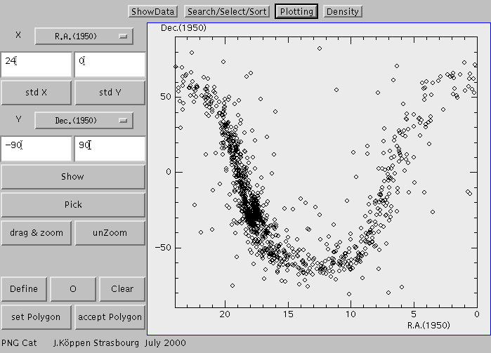
with the Choices for X and Y one may select whatever one wants to plot. Then, one clicks Show to actually show the plot. The text fields allow to enter the value for the left and right border in X and bottom and top for Y. If one wants to return quickly to the standard values for these ranges, one clicks the std X or std Y buttons.
To identify a certain object and to show all its data, click first the Pick button, and then move the mouse over to the object and click the mouse there. A new window with all data of this object will open. To close it, click on the window's O.K. button.
To zoom into any region of the plot, click Drag & Zoom then drag the mouse over that region of interest. Release of the mouse button will show the zoomed view. The unzoom button brings back the plot with the standard limits.
This page permits to select groups of objects by their geometrical location in the plot. There are two methods: Selection by rectangle or by arbitrary polygon.
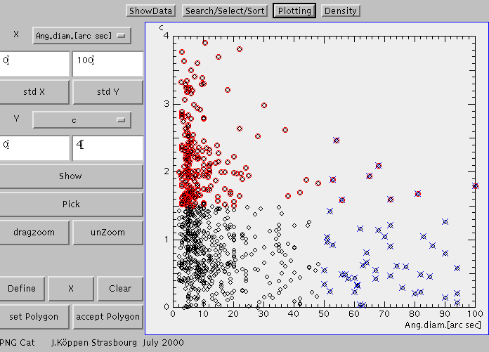
With the aid of these three symbols, one can define three groups, and the objects will be marked as belonging to these groups in every plot and also in the display of their data.
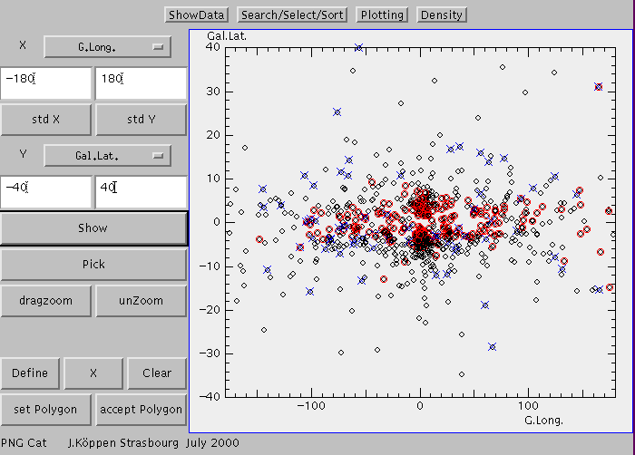
As an example, I have made two selections: red are objects with high interstellar extinction, and blue are those with a large angular diametre. Showing all objects in Galactic coordinates, one sees that the high extinction objects are concentrated to the Galactic plane, while the large objects are widely scattered over the sky.
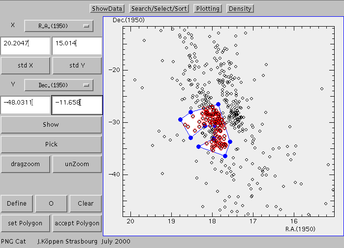
The choice by polygon is shown here, in a zoomed view. As before, one first chooses one of the three symbols O, X, or +. Then, after a click to set Polygon one clicks with the mouse at a number of positions in the plot to mark the corners of the polygon. It is best to start with just three points. Further points can be added to any side of the polygon; I recommend to move a newly entered point just a wee bit; this will cause the current polygon to be redrawn, and in this manner one does not mess up the relations of new point to its neighbours (I plan to improve this entering of points!)
The points can be grabbed and moved about. The number of points is not really limited, so any weird shape can be designed, even separated islands connected with very thin dams. The colour of the interior of the polygon is intended to be a light colour, but I have noted that it depends on whether other programs running on the machine changed the colour table....
When the polygon has the desired shape, one clicks accept Polygon and the plot will be re-drawn with all selected objects marked appropriately:
The control button Density changes over to making a density map of the currently chosen plot window: Here I show roughly the same region as in the last plot. The page now shows a colour-coded representation of the density of objects:
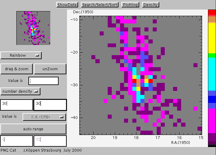
The small map at the upper left shows the full view, while the main area may show a zoomed view. This works with the drag & zoom and unzoom buttons in the same way as for the Plotting page.
A Choice allows to choose between different colour schemes. The current one is displayed as a thin bar at the right hand side, with the minimum (bottom; here: 0) and maximum (top; here: 13) values as given in the text fields in the lower left corner. Grey colour indicates that there is no object in the bin.
Clicking the mouse at any pixel of the main map will reveal the value at that location.
With a choice, one can choose to display number density or the mean value, dispersion, minimum or maximum of the value of any chosen column (see below)
The number of horizontal and vertical bins can be entered in the two text fields. When the CarriageReturn key is hit, the map will be redrawn accordingly.
Normally, the range covered by the colour bar is automatically scaled between the minimum and maximum occurring values. Clicking auto range defeats this option and allows to set the range by giving the values in the two text fields below.
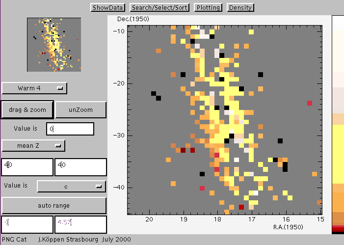
For the next screen shot, I had selected to show the mean Z, which enabled the Choice further down from which the column c was chosen. So this map depicts the distribution of the mean interstellar extinction of the objects seen in the sky (R.A. and Dec.) towards the Galactic Centre. One notes that the extinction increases towards directions closer to the Galactic plane.
Future plans: It is planned to add a page that allows to combine any columns by any mathematical operations. Furthermore, there will be a version - for the catalog manager - that allows to modify and edit any datum.
A catalog is organized in columns of various types which contain the data for each object. The catalog file is composed of two parts: first, there is a header with the descriptions of all the columns. In the second section we give for each object all its data.
The overall principle of the file is that each datum (a string, an integer or floating point number) is separated from the next by a carriage return. While this does not make the file easily readable for a human, it is necessary for being read by CatPlot.
First, the header containing the description of the catalog's structure At the beginning, any number of lines starting with "#" are comment lines and are ignored.
In the sequence of their occurrence, each column of the catalog is described by a number of items:
In addition, I have introduced for convenience some specialized columns:
This section terminates with:
Then follows the section with the data given for each object:
first, a string = the name of the object as a string then, in the same sequence as the columns were defined (above), their data must be given. the sequence depends on the type of the column:
A small nonsense sample catalogue can be seen here. This is the ascii-file small.cat which you can load into the applet when you start.
x-y data files are ASCII files which contain the data for the x-y plots in this format:
At the beginning, any number of lines starting with "#" are comment lines and are ignored.
Here is a most trivial example file.
Suggestion: If the upper or lower limit of the plot range are non-positive numbers (zero or negative) only a linear plot of that axis will be allowed. So if you have data between 0 and 12 and you want to make them also plottable in logarithmic fashion, it is better to specify as plotting limits 0.01 and 12.
To cut down transfer and loading times of larger catalog files, I use the Java binary format rather than ASCII. I have written a small Java application that converts an ASCII file myfile.txt into the Java binary myfile.bin. It is invoked by
java a2j myfile.txt myfile.bin
in the directory which must also contain these class files: a2j.class and Convertor.class. I'll make these files available. The binary version of small.cat is called small.cpb.
Converting ASCII xy-files into Java binary xy-files, and reading them, is a thing of the future.
| Top of the Page
| CatPlot Applet
| Index of my other Applets
|
last update: 12 May 2001 J.Köppen