Galactic Chemical Evolution in a One Zone Model
Joachim Köppen Kiel/Strasbourg/Illkirch April 2002
Contents
WithIn a galaxy, stars are born from the gas by gravitational instabilities. These stars live for some time, being powered by thermonuclear reactions in their centre which synthesize from the primordial elements hydrogen and helium all the other elements, such as carbon, nitrogen, oxygen, and iron. When the stars finish their lives either by exploding as a supernova of by expelling an planetary nebula, these thermonuclear 'ashes' are ejected into the interstellar gas, and are going to be used in the next generation of stars. In this fashion, the abundances of the heavy elements increase continually over the time, until there is sufficient of them available to make planets and create life.
The Applet computes this cycle of chemical evolution in a representative volume of a galaxy. This volume may be considerd as a closed system, where star formation consumes eventually all the gas. But also we can allow for an accretion (infall or inflow) of gas from another volume or from outside the galaxy, or for a mass loss by galactic winds. For both proceses, the user can input graphically how the rates should depend on the age of the system. The initial conditions (the amount of gas and its metallicity) can be changed. The recipe for the star formation rate - how it depends on the available gas mass - can be graphically given by the user. And how the production rates (yields) of two elements (called A and B) depend on metallicity (called Z) can be specified arbitrarily. The `element' Z is assumed to be produced with a constant yield by each stellar generation (`primary production'), and is used as a tracer of the overall evolution.
Any of the variables of the system may be plotted against another one, so their evolution in time, age, or redshift may be inspected, or the relation between two of them. The redshifts are computed with a Friedman type cosmological model, with the Hubble constant and the deceleration parameter. Furthermore, the distribution of the metallicity of the long-lived stars (`G-dwarfs') can be shown.
Some technical details: we neglect the finite stellar lifetimes (i.e. we use the Instantaneous Recycling Approximation) which is good for the elements produced only in the short-lived massive stars, such as oxygen. Elements produced in intermediate mass stars, such as carbon and nitrogen, or in type Ia supernovae (iron), cannot reliably computed with the applet! The equations are solved numerically with an automatically adjusted time step, which is controlled by the value given for the accuracy on the page with initial conditions.
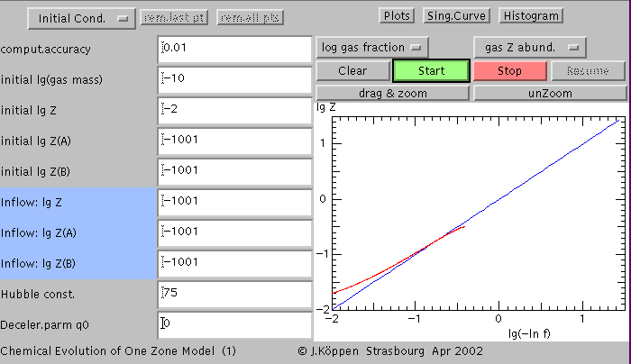
When you start up the applet, I recommend that you hit the Start button, and you see something like the following screen.

On the left hand side at the top, there is a Choice to navigate between the various input pages. It now says Initial Cond. which is the page just below. It contains mostly the parameters for the initial situation:
On the right hand side, at the top, there are three Buttons:
The page with the plots has several controls:
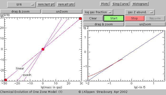
The plot shows the relation between the lg(-ln f) which is a
weird but useful form of the gas fraction
The red dots connected with red lines are the chosen recipe for
the star formation rate: the linear relation was chosen.
You may move a dot to a different position by grabbing it with
the mouse and dragging it over. Also, clicking at an empty location
will place a new dot there.
On the top there are two buttons which have become enabled:
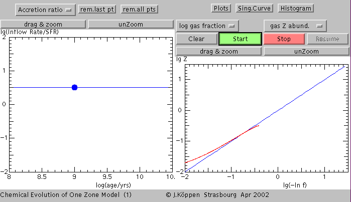
Chosing the Accretion Ratio brings this page:
which is another interactive plot showing how the ratio of the
rates of infall (= accretion = inflow) and star formation depends
on the age. Here we had chosen a constant ratio of 3.16.
Linear Accretion Model thus the evoltuion stops at
Z = 0.316 y
There are three more input plots: for galactic winds, and for
the nucleosynthesis recipe of elements A and B.
see below
But let us explore a bit further the
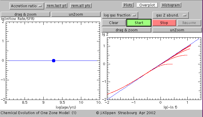
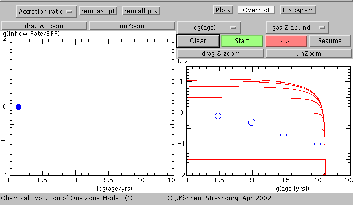
Linear Accretion Models: This is a plot with the
superposed curves from all models with accretion ratios
0.01, 0.03, 0.1, 0.3,1.0 etc. They show that the metallicity towards
which such a model tends, is the inverse of the accretion ratio:
The next screen shows the age-metallicity relationships
from these models, from which the saturating metallicities
are even more obvious:
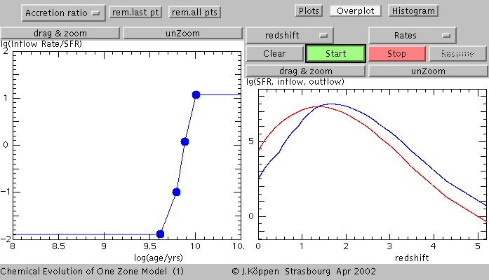
The next screen shows how some arbitrary history of the
accretion ratio results in a relation between star formation
rate (red curve) and accretion rate (blue) with redshift:
Obviously the earlier accretion causes an accumulation of
gas which then is comsumed to make stars. The SFR peaks
at lower redshifts than the accretion rate.
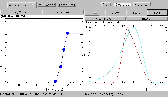
For the same model, we show the stellar metallicity histogram
(red curve) in comparison with the histogram of the Simple
Model (cyan curve).
When one wants to display this histogram, one may select
In the model, we follow the abundances of three "elements":
Z is assumed to be produced with a constant yield, and we use it
as a reference metallicity. Elements A and B will be synthesized
with yields that depend in a user-defined way on the metallicity Z.
This is done with the pages Yield A and Yield B .
Initially, the yield of A is assumed to be constant ("primary" production),
while the yield of B depends linearily on Z ("secondary" production).
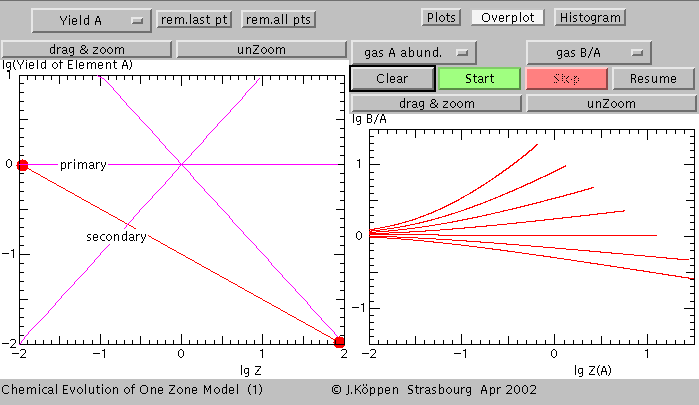
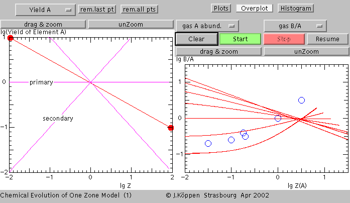
For the following screen, we made the yield of B constant (=1.0),
but we played with the yield of A: the left point is always kept at the
position shown (1.0), but the right point was moved from the top
(100) to the bottom (0.01) in half-decade steps. The plot on the
right hand side shows the effects of the various metallicity-dependent
yields for A in the diagram of abundance ratio B/A plotted against the
abundance of A:
We see that if A's yield declines with metallicity (as shown)
one gets the top curve, the B/A ratio increases with A.
This kind of diagram is used to judge on the nucleosynthesis
origins of the elements, usually one takes for element A one which
is produced with constant yield, such as the N/O vs. O/H plots.
But if the oxygen yield were not constant ...
For the screen below, we changed the slope of the yield, but keeping
the point in the centre (1.0, 1.0) fixed:
The blue circles are data used for an exercise.
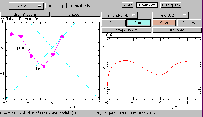
If one plays simply with the yield curve - without bothering about
its physical reality - one finds that this curve is quite well mapped
from the yield plot into the abundance ratio plot:
Apart from the units as shown in the plot axes, one word about
the unit of mass for the gas, stars, and the rates of star formation,
infall and wind loss:
There is no preferred unit, so one may think of one unit as
the entire mass of a galaxy, or its mass in solar mases,
or the mass contained in some given
volume (a cubic kpc ...). In models without inflow of gas, the
natural mass unit would be the mass initially present in the zone.
In models with inflow, it may be more practical to set the initial
gas mass to a tiny portion of the mass unit, and one may end up
with a final mass much greater than that unit. In the applet, the
ranges of the masses are taken rather large, in order to permit the
user to treat any problem one might like to investigate.
While the type of a model and its solution depends on certain
ratios of the rates (e.g. the accretion ratio) rather than the rates
themselves, the real values of the present star formation and
accretion rates are of interest. They depend on the assumed
mass unit: if one had chosen the mass of the galaxy, then the
proper rates are in "galaxy masses per Gyr", of course.
| Top of the Page
| Controls
| Applet
| Applet Index
|
The Units