Model Population of Stars
J.Köppen Strasbourg/Illkirch/Kiel May 2001
-------- under modernisation -----------
Contents
About the Applet and what it does
The luminous matter in the Universe is organized in galaxies
which consist of stars and interstellar gas. The stars have
been born at various times in the past from the gas by
cold molecular clouds becoming unstable against their own
gravity. Nearly all the optical brightness of a galaxy comes
from the present stellar population which thus may be a combination
of young and old, hot and cool stars. From theoretical work,
it is fairly well known how stars of the various masses change
with time, so it is possible to model a population of stars,
in order to find out how star formation occurred in the past.
Because star formation is something we still cannot derive
from basic physics. So one describes this process by assuming
that stars are born following a certain distribution
Function of their Initial Masses (the
IMF, usually decreasing like a power law with increasing
mass), and that the star formation rate (SFR) describes
how much gaseous matter is converted per time unit into any kind
of stars. The evolution of the new stars depends on the metallicity
of the gas out of which they were formed.
The StarPop Applet allows to
compute the theoretical and observable properties of single
stars of any mass and age and various metallicities. It also
permits to create synthetic populations of stars born with
any arbitrary history star formation.
A Tour around the Applet
This is how your screen should look like after the applet has
been loaded and started, and you have clicked Clear:
 There is a white plotting area and some controls on the top:
- Clear to >>>>
- will clear the plotting area to show the diagram whose
axes will be as indicated on the right:
- X = Teff (log)
- selects what is to be meant by the x-axis. Here, the
effective temperature of the star(s) is chosen. The
(log) indicates merely that the axis will be divided
in logarithmic fashion, which is useful for the large
range of temperatures that need to be shown
- Y = lg(L)
- ditto, for the y-axis. Here, the logarithm of the luminosity
(in units of solar luminosity) is chosen
These controls are accessible in all the pages.
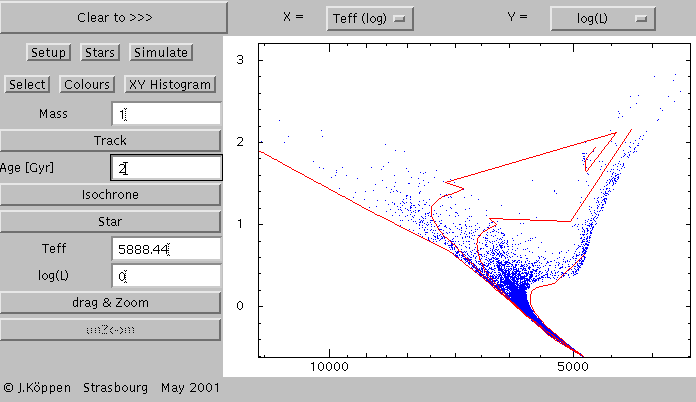
There are quite a few controls on the left hand side. At the top
the principal buttons Setup, Star,
Simulate, Select, Colour, and
XY Histogram are placed. These are used for
navigating in the applet. Right now we are in the Star
menu, and beneath we find all its revelant controls:
- Mass
- here one enters the mass of the star (in solar masses)
- Track
- clicking this button will plot as a blck curve the
evolutionary track of the star with above given mass
until the age given below
- Age [Gyr]
- the age of the star, or the maximum age of a star on
its track
- Isochrone
- clicking this button will plot as a red curve the position
of stars of all masses, but of a given age
- Star
- clicking this marks with a black dot the position of the
star with given mass and age ...
- Teff
- ... for which the effective temperature will be shown ...
- log(L)
- ... as well as its luminosity
- drag & Zoom
- click the button and drag (move while keep the button
pressed) the mouse over any area of the plotting screen
will select this rectangular area for the new view.
Note that everything plotted before will be wiped, and
you'll have to re-draw
- unZoom
- brings back the default view of the plot
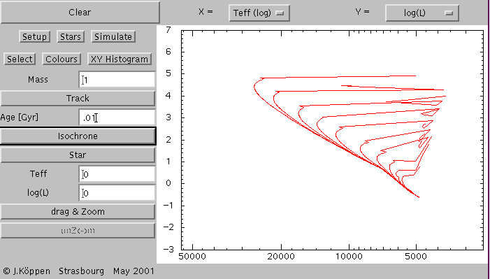
 Here we have plotted the isochrones for ages of 0.01, 0.02, 0.05,
..., 2, 5, and 10 Gyrs (from left to right).
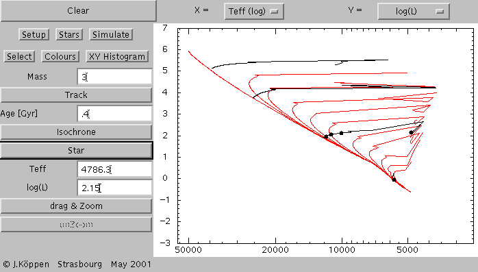
 And here we added the evolutionary tracks of stars with 1, 3, 10,
and 30 solar masses (black curves), the zero-age isochrone (red curve),
and the positions (black dots) of a 3 solar mass star at ages
of 0.1, 0.2, 0.3, and 0.4 Gyrs.
The effective temperature and luminosity of the last position
is shown in the text fields.
Also shown is the position of a 1 solar mass star at an age of 3 Gyrs.
 Now the area near the present solar position is zoomed by using the
Drag & Zoom button and dragging the mouse over a suitable area.
One may zoom as deeply as one wishes, however the labels
on the axis tick marks will eventually disappear, and one may also
rather quickly notice the effects of linear interpolation in the
evolutionary track data!
The unZoom button will always bring back the overall
view.
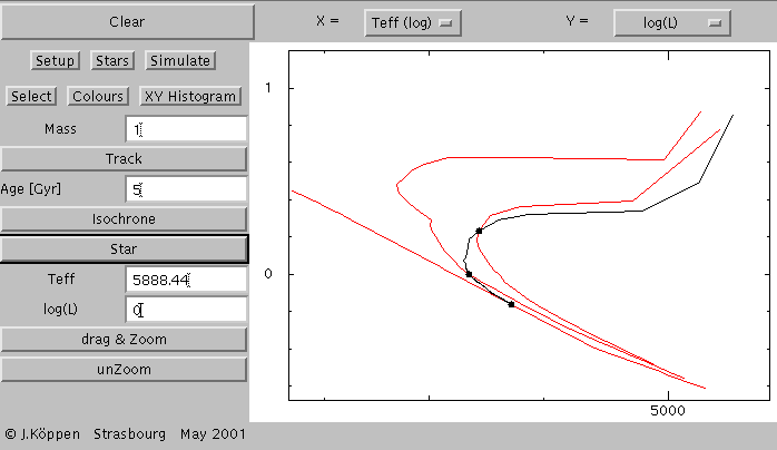
All graphics will be erased, and we show the isochrones for
0, 5, and 10 Gyrs, the complete track of a 1 solar mass star
(specifying 20 Gyrs age), and the positions of the sun at ages
0, 10, and 5 Gyrs, the latter's temperature and luminosity are given.
So far, we showed only the normal Hertzsprung-Russell diagram.
The Choices at the top permit to select any two of the following
stellar parameters as X- or Y-axis:
- Teff (log)
- effective temperature
- log(L)
- log of luminosity, in solar units
- R* (log)
- star's radius, in solar units
- M* (log)
- mass, in solar units
- log(g)
- log of the star's surface gravity, in cm/s^2
- age [Gyr]
- star's age, shown in linear scale
- age (log)
- age, but in logarithmic scale
- U
- brightness in the U-band (about 365 nm wavelength),
in magnitudes
- B
- brightness in B-band (440 nm)
- V
- brightness in V-band (548 nm)
- U-B
- colour index = difference of U and B magnitudes
- B-V
- colour index
- SFH
- Star Formation History, the star formation rate
as a function of age
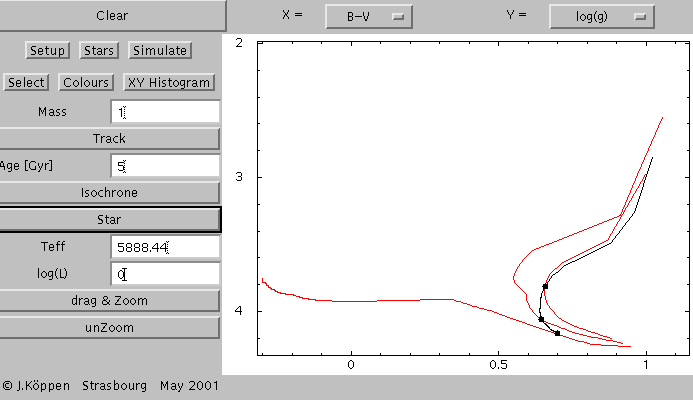
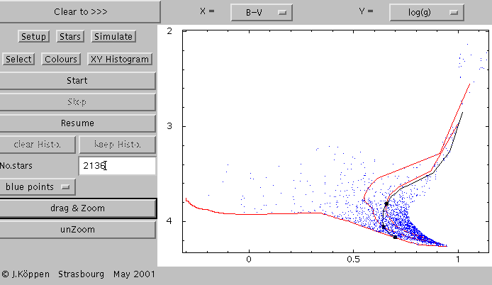
 This is the same set of curves as before, but in the diagram of
B-V colour index against the surface gravity g, also zoomed
to bring out the interesting parts.
 From the last picture, we've switched over to the Simulate
page. This has these controls:
- Start
- starts a Monte Carlo simulation
to create stars with certain mass spectrum and certain
star formation history
- Stop
- halts the simulation
- Carry on
- continues with the simulation.
- Clear Histo.
- clears any simple histogram we
may have kept from earlier simulations
- keep Histo.
- keep the present histogram
in memory, and superimpose it with any further results
- No. stars
- shows the number of stars
simulated so far
- blue points
- allows to change the colour
of the plotting points: red, blue, green, black are available
- drag & Zoom
- click the button and drag (move while keep the button
pressed) the mouse over any area of the plotting screen
will select this rectangular area for the new view.
Note that everything plotted before will be wiped, and
you'll have to re-draw
- unZoom
- brings back the default view of the plot
Let us now click the Start button, and after a while the
Stop: We have created a stellar population of about 2000
stars, whose positions are indicated as blue dots. We'll return to
this later, but what is behind all this?
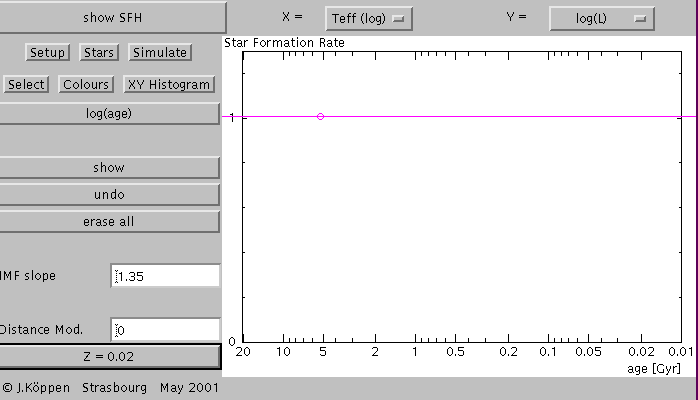
 This is shown by the Setup page. It displays the star
formation history only, and has these controls:
- log(age)
- switches between linear and
logarithmic scale for the age axis
- show
- just refreshes the plot
- undo
- removes the data point entered last
- erase all
- removes all data points
- IMF slope
- shows the exponent of the power-law
function assumed for the distribution of initial masses
of stars in a population. 1.35 means the Salpeter law,
i.e. the mass contained in stars with masses between
m and m+dm decreases like the 1.35rd power
of m
- Distance Mod.
- the distance modulus for
the population.
- Z = 0.02
- metallicity assumed for the stellar
evolutionary tracks and the photometric colours.
Z= 0.02 means that 2 percent of the mass of a piece
of the star is in the form of 'metals', elements heavier
than helium. This is the solar value.
Z = 0.001, 0.004, 0.008, 0.02, and 0.04 are available
From this we see that in the present simulation
the star formation rate is taken as being constant for all ages
(from 10 million to 20 Gyrs), that solar metallicity (Z=0.02) had
been assumed for the evolutionary tracks. And that the
IMF slope was 1.35, i.e. we had assumed a Salpeter initital mass function.
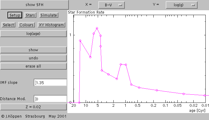
 Let us first play with the star formation history: Just click with the
mouse on the plotting screen. A small mauve circle will mark
the datum. One can grab the circle and move it about. If you are in
what is the current SFH, click either Clear SFH,
show, or merely move one of the data points a bit.
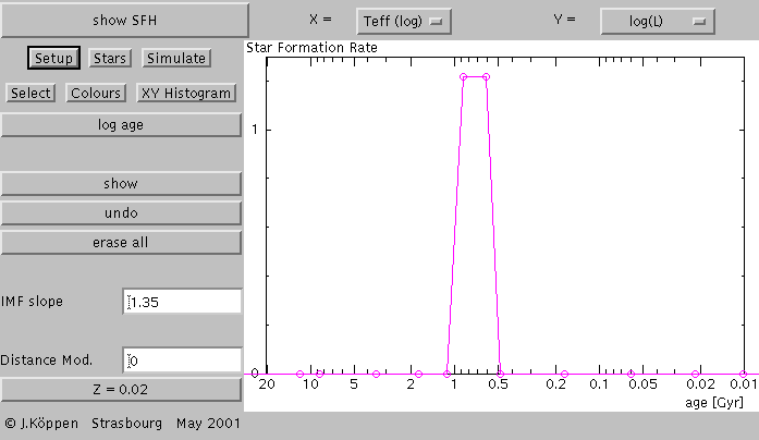
Let us here assume
that on some background rate which increases with age - because
in the past there was still more gas available to make stars than
today, and of course no star formation before the Big Bang (about
15 Gyrs ago) - we put one star burst, about 1 Gyr ago:
 This is what we got from the simulation:
We have overlaid the simulated Hertzsprung-Russell Diagram
with the isochrones of 0, 1, 2, and 13 Gyrs. We can see that just
to the left of the 1 Gyr isochrone the stars are more numerous.
But also that the diagram is still dominated by the underground star
formation.
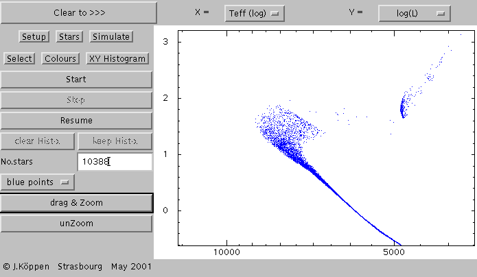
 To isolate the effects of the different populations, we can
first regard the burst with the above star formation history...
 ... which makes this zoomed HRD. Now - do NOT click
the Clear button! - let us go back to the Setup page
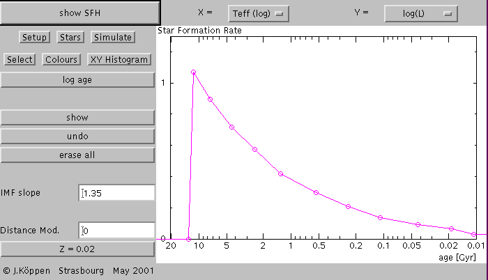
 and compose the underlying star formation
Then we go back to Simulate page - again: do not press Clear!
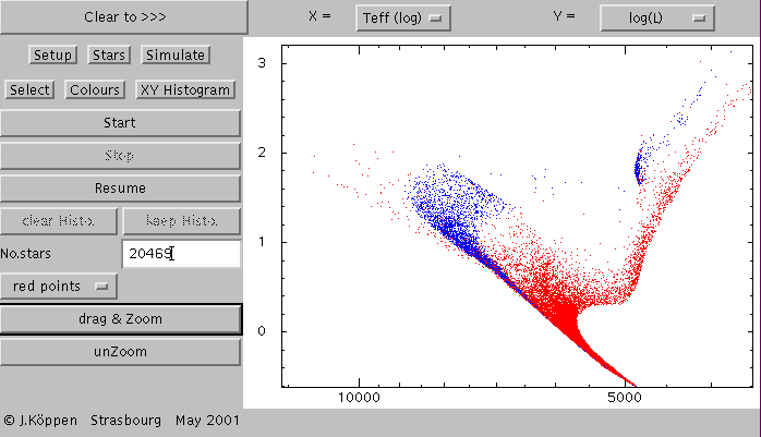
Here we first change the colour of the points from blue to say: red,
and then we click Start button. This will add the second population
to what was on the screen. If we run this for a while, say up to
twice as many stars we had in the burst population, we
get this
 where we can easily identify that the burst population will dominate among
the hot stars - only few are produced in the background population,
it will also contribute to the red giant stars, but the older background
population dominates both among the red giants and the fainter
stars close to the main sequence.
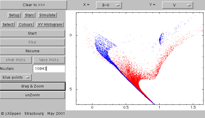
 What we observe directly is the colour-magnitude diagram, e.g.
B-V against V, done for the same populations
which indicates that one could discriminate between the populations
in a histogram of the B-V colour indices.
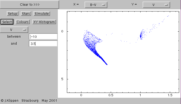
 But before we make the histogram, let us select only stars which are
brighter than say 6.5 magnitudes in V. This is done on the Select
page, Its controls are:
- no selection
- this Choice allows to choose
one parameter for whose values the simulated stars
will be selected
- .......
- the text fields specify the lower and upper
limit of the acceptable values. Note that we mean numerically
upper and lower value, i.e. when stars brighter than 5th
magnitude should be accepted, one specifies -100 and 5!
and the above plot shows the result of the simulation of the burst
population.
You may have noticed that the Choice for the Y-axis also has an
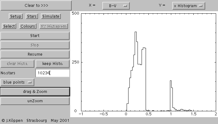
entry Histogram. When chosen, a histogram of the
parameter selected for the X-axis will be done:
 This is the histogram of B-V colour from 10000 stars of the burst
population.
As the histogram builds up, the picture is automatically rescaled
whenever the peak values become sufficiently large.
By clicking the keep Histo. button we save
this curve.
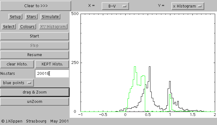
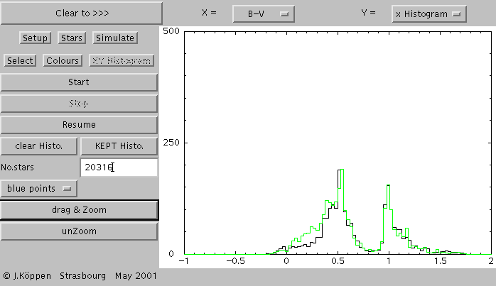
 And this is what one gets for 20000 stars from the background
population, this is shown by the black curve, while the
green curve shows the saved histogram of the burst population,
scaled to the same maximum value.
 Here we compare the 30000 stars of the composite star formation
history (green histogram; oh yes, one had to enter this in the Setup
page) and 20000 stars of the background only (black).
The two histograms are very similar, but the composite population
has more bluer stars, with colours B-V between 0 and 0.5.
One has to look carefully, if one has only colours.
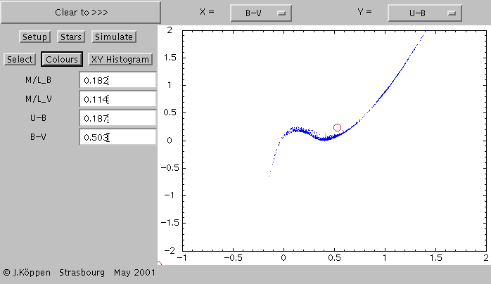
One can also get the integrated colours of the whole population.
While a simulation is going on, one may click the button for the
Colour page and every 50 stars, the colour indices U-B and B-V
as well as the ratios of mass-to-luminosity in the B and V bands
are displayed. So one can watch until the numbers are sufficiently
stable, and stop the simulation. When the two-colour diagram
X=B-V and Y=U-B are selected, a red circle appears to show the
integrated colours:

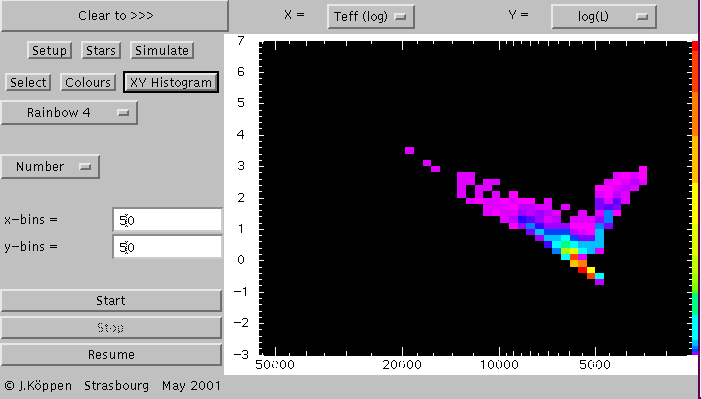
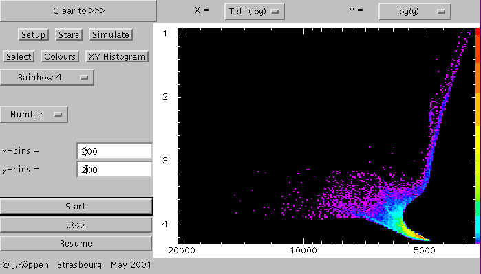
Finally, we can show all diagrams also as a colour-coded
plot of the number density of points in each area of the diagram.
This is the XY-Histogram
 Here is the plot for the composite population, now with the
selection in V magnitude again switched off.
The controls are:
- Rainbow 4
- selects the type of colour coding,
such as Raimbow, White-on-Black, Black-on-White, Warm.
The number indicates with what power law the coding is distorted,
as to emphasize the large values (-4, -2) or the small values
(4, 2). In any case, the current color bar is displayed as a narrow strip
to the right of the plot area, showing the coding between 0 (bottom)
and 100 percent (top).
- Number
- selects what is shown by the colours:
the number density, or weighted with the mass, luminosity, U-,
V-, B-luminosities, or the B-V or U-B colour indices.
- x-bins, y-bins
- give the numbers of bins
for the x- and y-coordinates. More bins give finer resolution,
but also require more time to paint the plot.
There is no limit to the number of bins one may employ; the main
limitations are the available space on your machine and your patience
to seen all points to redrawn.
- Start
- starts the simulation ...
- Stop
- ... halts it ...
- Resume
- ... continues with the current simulation
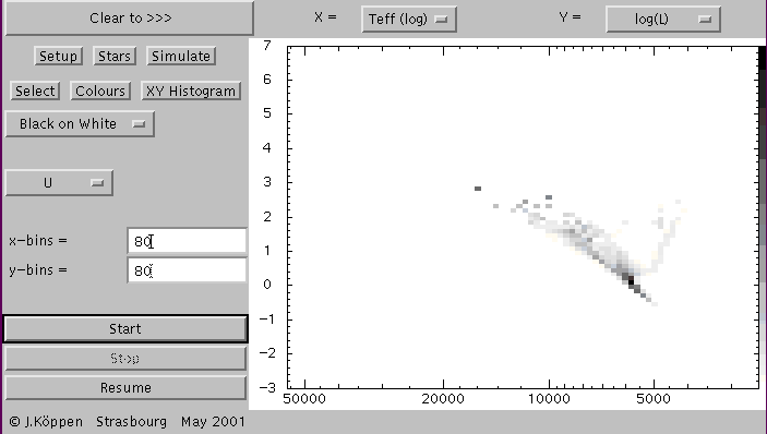
Weighting with U-luminosity
shows the Hertzsprung-Russell Diagram for our population,
here in a gray-scale representation.
 The hot main sequence stars contribute much because of their
luminosity and temperature, but the cooler main sequence stars
also contribute because of their large number. Red giants are
not strong contributors to the U-luminosity.
As the histogram builds up, the picture is automatically rescaled
whenever the peak values become sufficiently large.
The XY-Histograms can also be done for a zoomed view: zooming
is done from the Star or Simulate pages.

Some Experiments
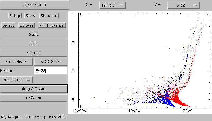
Here is a view of a portion of the Hertzsprung-Russell diagram in
the form of effective temperature and surface gravity: the blue dots
are stars of very low metallicity (Z = 0.001), the red ones have
solar metallicity.

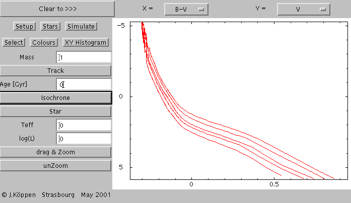
This plot shows the
zero-age isochrones of all metallicities 0.001, 0.004, 0.008, 0.02, and
0.04 (from left to right). The curves are not smooth curves in the
upper left hand corner. This is because of our rather simplified
interpolation of the colour corrections.

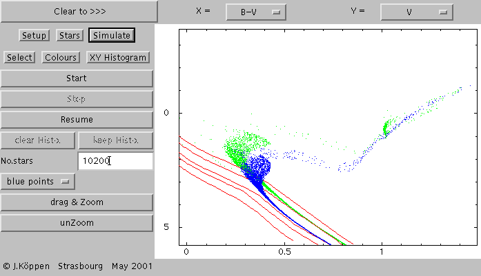
The zero-age isochrones (in red) are overlaid with two stellar
populations:
In green, a solar metallicity, 1 Gyr old population, in blue
one with roughly half metallicity (Z = 0.008) but twice as old.
The integrated colours are quite similar, showing the age-metallicity
degeneracy.

Details:
The applet uses the theoretical evolutionary tracks computed
by the Geneva group.
The photometric colours are computed using tables calculated
with the Kurucz' grid of theoretical stellar spectra.
The initial mass function (IMF) is assumed to be is a power law in
the range of stellar masses between 0.8 to 120 solar masses.
The value of the exponent of 1.35 refers to Salpeter's IMF.
| Top of the Page
| Controls
| Applet
| Applet Index
|


