Finding the Spiral Arms of the Galaxy
Joachim Köppen Strasbourg 2010
To find the spiral arms of the Milky Way, we first have to do
a complete survey of the Galactic Plane. From the Northern Hemisphere
we can only observe Galactic longitudes between about l=0° and l=240°,
that's three quarters. For every position in the Plane, we should get
a good spectrum, covering radial velocities between -150 and +150 km/s.
Since the antenna's HPBW is about 5°, it would be quite sufficient to
observe every 5°, but it does not harm to cover the Plane with a finer
stepwidth, because one would execute these observations by
batch operations. At every position, we should
collect a sufficient number of good spectra, from which we can obtain
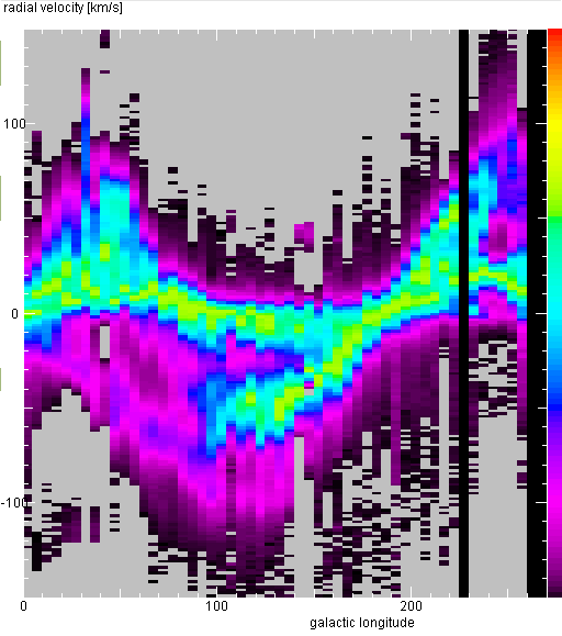
a good quality average spectrum. Plotting these average spectra as a
function of galactic longitude in the same way as we plot the
waterfall map of any data,
we would get a false colour map like this:
 For the analysis, such a plot is very nice, but you can also deduce
the spiral arms by simply looking at the averaged spectra for each
longitude (see below).
We can see that at some position there are distinct emission features
at several different radial velocities. These features can be traced
over a large range of longitudes. Each such feature is emission coming
from the hydrogen gas in a spiral arm. They are quite distinct, so let
us try to identify them and trace them in the Galaxy.
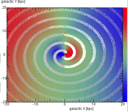
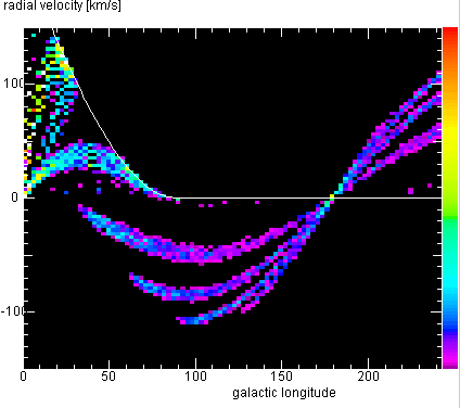
The JavaScript tool:
Modeling of the Spiral Arms in the Milky Way
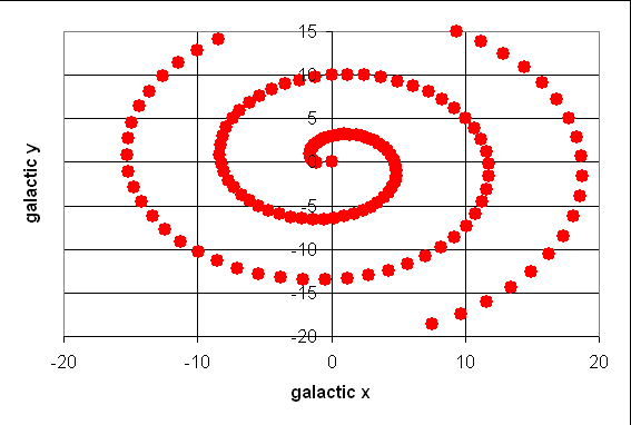
allows you to construct a model of the spirals in the Galactic Plane,
such as depicted in the left hand image below,
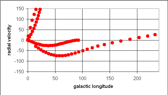
and then you can show how the emission by the spirals would look like
in the longitude-radial velocity map (right panel)


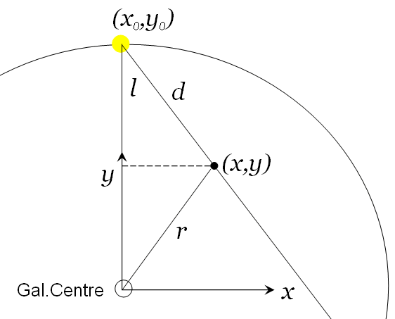
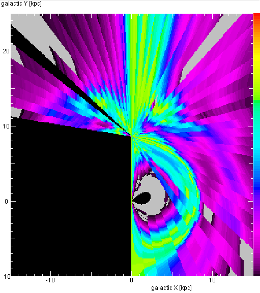
What is behind this tool, and behind such an analysis? The rendering below
shows our situation in the Galactic Plane:
 The Sun is at a position x0=0 and y0=8.5 kpc. When we look at
Galactic Longitude l, we get emission from any distance d
on the line of sight indicated. Therefore we can compute the position
x,y of that point
x = x0 + d sin l
y = y0 - d cos l
From this, we know its distance from the Galactic Centre
r = sqrt(x˛ + y˛)
Let us assume that we have determined the rotation curve, or that we simply
guess it by the rotational speed v0 = 220 km/s at the position of the
Sun, and the slope dvdr = 0 km/s/kpc, say, with which it increases with
distance from the centre. So we can compute the rotational speed at that
point in the Galaxy
vrot(r) = v0 + dvdr (r-r0)
Finally, ff one works out the radial velocity of this point as the projected
rotational velocity, one obtains Oort's equation
vrad(l,d) = (vrot(r) r0/r - v0) sin l
This means that we can associate each position given by Galactic Longitude and
distance with a spot in the Longitude-radial velocity diagram. However, the
inverse is not generally true: As explained in
Galactic Rotation, on any line-of sight towards the
interior (|l| < 90°) there are two distances whose emission appears at
the same radial velocity. Thus, we cannot attribute a single distance to a specific
radial velocity. But nonetheless, we can map our observed longitude-radial
velocity plot into linear galactic positions:
 We can distinguish two or three spiral arms: the one in which the Sun is located,
one further out, at about 12 kpc distance from the Centre, and perhaps another
one even further out. Perhaps there is another one inside the orbit of the Sun,
but note the ambiguity for this inner part!
However, such a direct mapping is a bit complicated to program, and one has the
ambiguity for the regions inside the Sun's orbit. Therefore, it is better and more
comprehensible to do the analysis in the forward way: assume some spiral pattern
and try to match with it your observed l-vrad map.
One can use this tool: Modeling of the Spiral Arms in the Milky Way
There is another, even simpler way, which can be implemented even in Excel:
- create a table with the first columns of longitudes and distances;
put in a number of points, with guessed or random data
- make a scatter plot (with symbols only) of this table, but specify the data
region as having more rows
- say 50 or 100 - than you had already filled with data! It is a good idea
to mark all these rows with some background colour.
- now add more columns to this table: using the above equations, compute
successively: x and y, r, vrot, and vrad.
Do this in the first row, then copy the formulae to all rows you had
marked by colour.
- make a scatter plot (with symbols) of the columns longitudes and
vrad, and
force the plot range to be the same as your observed l-vrad map. Use a nice
symbol, such as an X or an open circle. And also, include all coloured rows
in this plot.
- now you can modify or add more points by entering their longitude and
distance, to make the points in the l-vrad plot to match the positions
of observed emission
- you can also grab a symbol in the l-d plot and move it in one direction ...
so you can almost interactively adjust the positions in the l-vrad plot.
- when you are done, you can make a third scatter plot with symbols, this
time for the x and y columns. The symbols show you the distribution of
emission as if you looked down on the Galactic Plane.
Important note
For this analysis it is not really vital to make a false colour map of longitude
and radial velocity ... Simply inspect your averaged spectra at each longitude,
identify the features, and try to match the measured radial velocity by guessing
the distance, with the longitude being given.


| Top of the Page
| Back to the MainPage
| to my HomePage
|
last update: Feb. 2010 J.Köppen
