Performance of Parabolic Dish Antennas
Illuminated by Various Feeds
Joachim Köppen DF3GJ ... Kiel, March 2020
Some brief explanations
This tool computes the properties of circular dish antennas, illuminated by various feeds. It is based on the program FeedPatt by Paul Wade (W1GHZ, ex-N1BWT) and uses the data files from his W1GHZ on-line microwave antenna book and found on his website. It has been tested to work on Firefox, Edge, and Chrome, and partially with InternetExplorer.- On the left is a panel to enter various parameters of the antenna and select the Feed and the Display for the results (see below).
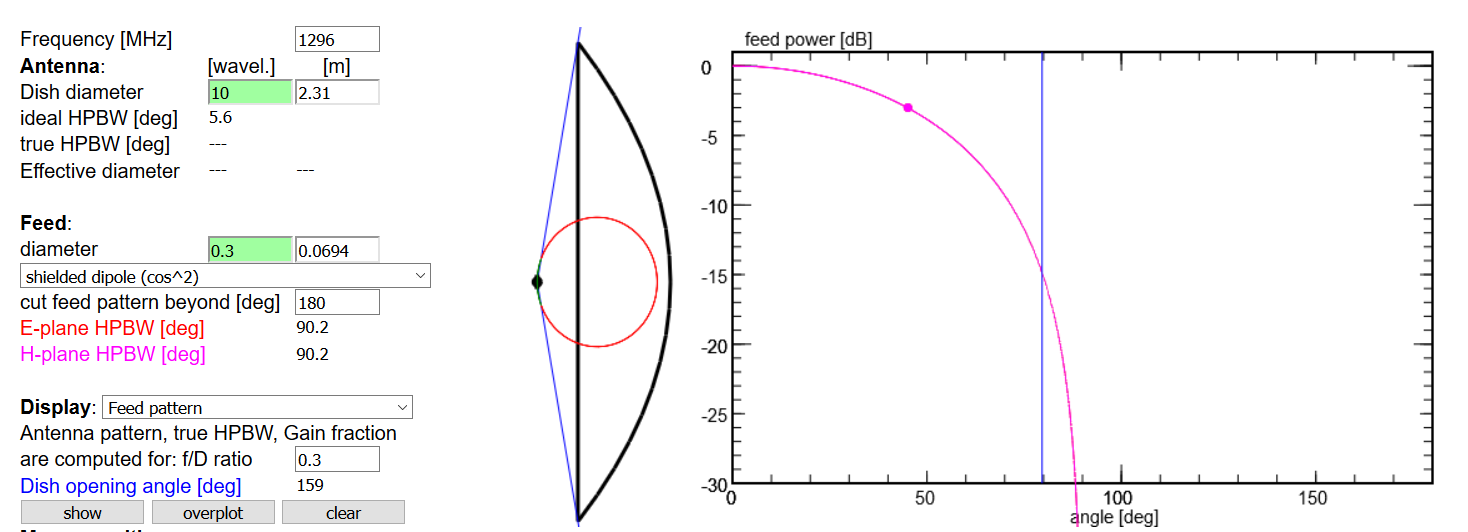
- The middle panel gives a view of the antenna (in black outline), the focal point (black dot), and the radiation pattern of the selected feed. The red part of that curve is what illuminates the dish, the green part is what does not reach the dish and which constitutes the spill-over losses. This curve indicates the power radiated by the feed in linear units. A black bar at the focus shows the size of the feed. The blue lines indicate the range of angles seen from the focal point which is covered by the dish reflector.
- The larger panel at right contains the plots of the results:
- Feed pattern displays the radiation pattern of the selected feed antenna: The red curve is the pattern in the E-plane, and a red dot indicates the HPBW. The magenta curve is the pattern in the H-plane. For some feeds both patterns are (assumed to be) the same, and only a single magenta curve is seen. A blue vertical line marks the angle up to which the dish fills the view from the focal point.
- Dish illumination displays the illumination on the surface of the dish. The red curve is the pattern in the E-plane, the magenta curve is the pattern in the H-plane. For some feeds both patterns are (assumed to be) the same, and only a single magenta curve is seen. A blue vertical line marks the other rim of the dish.
- Efficiencies shows several things:
A red curve is the fraction of the feed power that ends up in the beam. Thus it is the feed efficiency, but it may be taken as an indication for the overall efficiency of the antenna, as a function of the f/D ratio of the antenna's focal length and diameter.
The green curves indicate the fraction of the feed power that does not reach the dish, and is therefore lost as spill-over. The full line is the total spill-over. Long dashes indicate the spill-over to angles higher than 90° from the main beam direction, and thus towards the rear of the dish, which is important because of the pickup of thermal noise from the ground. Shorter dashes are the spill-over to the sides, to angles between 30 and 90° off the main beam, and usually not too important unless high trees or buildings block the sight. Very short dashes is the spill-over to the front, within 30° of the main beam, obviously of little importance, as one would pick up noise from the sky. The curves are marked by the letters B, S, and F.
The grey curve shows the illumination loss (1-b/d), where b is the power in the beam if there was no blocking by the feed, and d is the power deposited on the dish. It thus indicates how well the dish is illuminated.
The magenta curve gives the illumination at the edge of the dish. This is in linear units, so that the recommended value of -10 dB corresponds to 0.1.
The top of the plot contains marks of the opening angle of the dish as seen from the focus. Red, green, and grey dots indicate the curves' values for the f/D value chosen on the parameter panel at left, thus representing a specific antenna configuration. - Gain fraction shows how much of the total gain of the antenna is contributed by which part of the dish. Since the reflecting area increases with radius, the central section within 10 percent in radius contributes very little, but the outer rim with its much larger area supplies much more. The steeper the curve, the larger the contribution. The top of the plot contains marks of the opening angle of the dish as seen from the focus. A black bar near the top shows the size of the feed which causes shadowing. Note that this plot is done only for the the f/D value specified on the parameter panel at left.
- Antenna pattern gives the radiation pattern computed for the
dish antenna illuminated by the chose feed, and for the specified
f/D value. It also takes into account any shadowing by the feed.
It does not distinguish between the E-plane and the H-plane, so the
pattern is rotationally symmetric about the axis in the direction
of maximum signal ('optical axis').
Several parameters are displayed: the antenna solid angle ΩA,
the beam efficiency ηB = ΩB/ΩA,
spillover, illumination loss, edge and feed taper.
As this computation takes a bit of an effort, be patient for a few seconds ... The red dot is the resulting true HPBW of the antenna, which is also displayed on the left panel. Note that the true HPBW can only be shown after making this plot (and the necessary computations). - The left panel contains input parameters and results:
- Frequency
- Dish diameter: this can be entered either in wavelengths or in meters, whichever field is shown in light green. Simply enter your value in the appropriate field and hit the Enter key. This will change to the chosen option, and the other value is computed from your value.
- ideal HPBW: is computed for a uniformly illuminated dish of the given diameter (note that while for a 10 wavelength diameter dish the theoretical value for the HPBW is 58.957°, we rather use 56° to match results from the numerical computations used in this tool)
- true HPBW: is computed only when the 'antenna pattern' plot is shown for the chosen feed and specified f/D ratio.
- Effective diameter: is the diameter of a uniformly illuminated dish with the same HPBW as the true value.
- Aperture efficiency: is the ratio of effective area to the geometrical area of the dish (= square of effective and geometrical diameters).
- Collar height: is the height of a cylindrical collar around the dish's rim.
- Feed diameter: (a) in the efficiencies plot, the overall efficiency
also takes into account the shadowing by the feed.
(b) the theoretical feed pattern (e.g. uniform cone) depend on the dimension of the feed. A larger feed results in a narrower pattern. - Choice of the feed:
... there are several simple theoretical patterns and numerous data files from W1GHZ of simulated or measured patterns.
... Read data from User computer displays a field at the top of the page. Click this or the 'Browse...' key to open a file selector window that allows you to choose a file on your computer. [This option does not work with InternetExplorer].
... Read data from input page takes the data that may be entered in the text area on page 'Input: Feed Pattern' - cut feed pattern beyond: this option allows to cut the pattern of any given feed for angles larger than the specified value.
- E-plane HPBW: is the feed's HPBW in the E-plane.
- Display: here you navigate among the plots.
- f/D ratio: this can be specified in order to model a specific antenna configuration. The value affects the antenna pattern, the true HPBW, and the gain fraction plot.
- Dish opening angle: is the angle under which the entire dish is seen from the focus.
- Show: displays the last results again.
- overplot: click this, so that the button is lit light green. Then all following plots - by changing any parameter, or choosing another feed - will be superposed, for a direct comparison.
- clear: wipes any plot.
- The mouse position gives the coordinates of that point, allowing to read numerical values from the plot. In some browsers, these values may not correspond to the plot. If this happens, keep this page in its initial top-left corner position.
| Top of the Page | Java Applets Index | JavaScript Index | my HomePage |
Hint: a click on an image will show it full size in a new tab.
In all operations on the Compute & Display page, we first give the Frequency and the Dish diameter of the antenna. We may specify the diameter in wavelengths or in meters. Hit the enter key after you entered the number in the chosen field, to make this field green to confirm your choice.
Then you will find below the ideal HPBW, which is for an uniformly illuminated circular dish. The true HPBW and the effective diameter are computed and displayed only when you had chosen to display the antenna pattern.
Then you give the parameters of the Feed: Specify its diameter (we assume that it is of circular shape, too), and choose among a list the type of feed. This list contains:
The HPBWs in the E-plane and the H-plane are displayed. Note that some patterns are only given in the E-plane, including the data from the Input page or from the User computer!
The sketch left of the plot shows the true geometry of the antenna and feed, with the feed pattern (red curve) and the opening angle of the dish as seen by the feed (blue lines).
Common to all plots is the display of the current coordinates of the computer mouse, which are displayed at the lower left corner.
Next, chose the Display:
The plot shows the pattern of the feed antenna: if the pattern is available in both E- and H-plane, the red curve displays the E-plane pattern. Otherwise, a single magenta curve shows the feed pattern. The dot on each curve indicate the feed HPBW in the corresponding plane. The vertical blue line marks the angle to the dish's rim; thus, the power in the part of the pattern that extents beyond this angle is lost by spill over.
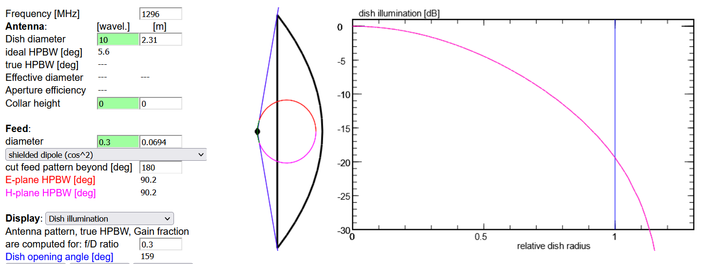
The plot shows how the illumination varies over the dish: if the pattern is available in both E- and H-plane, the red curve displays the E-plane pattern. Otherwise, a single magenta curve shows the feed pattern. The vertical blue line marks the outer rim of the dish; thus, the power in the part of the pattern that extents beyond this radius is lost by spill over.
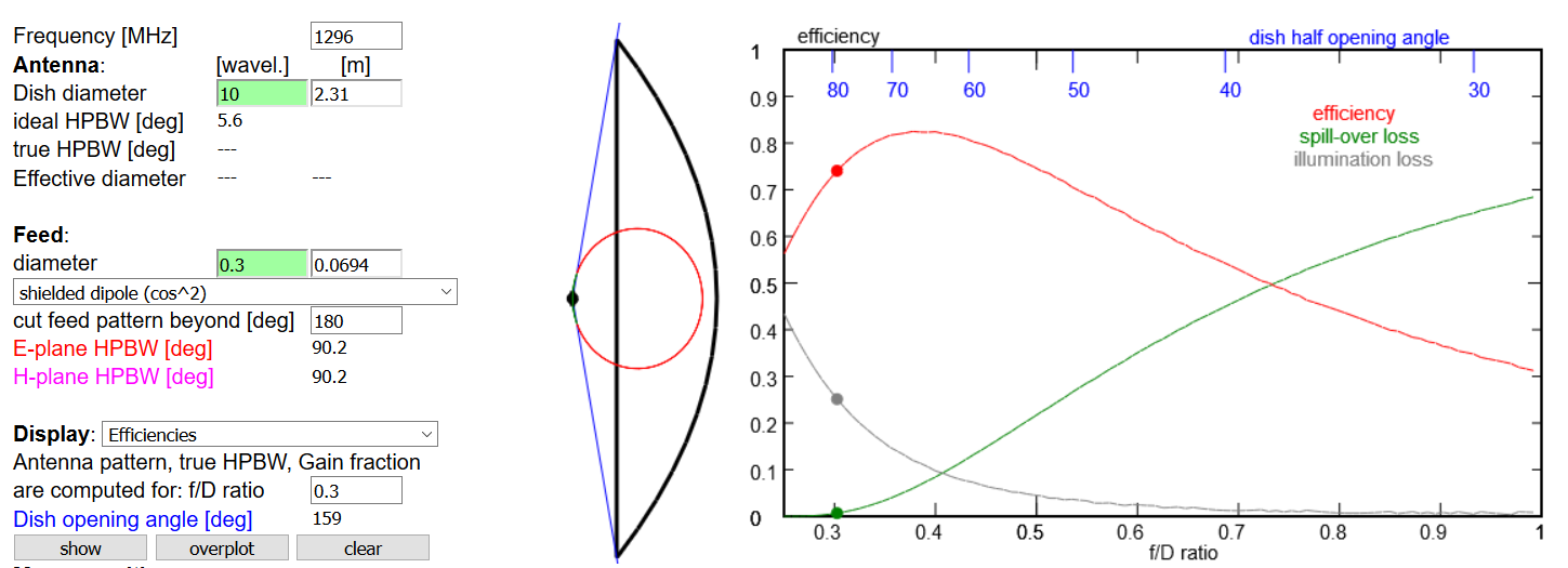
This plot shows the same quantities as the plots in Paul's book, as functions of dish f/D ratio. The red curve is the feed efficiency, i.e. the fraction of the power fed to the antenna which is actually radiated into the antenna beam and thus in the desired direction. Like in Paul's program, this and the other quantities are computed by taking the mean of the E- and H-plane amplitudes at each angle as the amplitude which illuminates the dish. The green curve shows the spill-over loss, i.e. the fraction of feed power that is radiated beyond the dish's outer rim, and thus is not available for being focussed into the antenna beam. The grey curve is the illumination loss which is a measure of how much the dish differs from the ideal of fully illuminated antenna. The dots in the curves mark the currently chosen f/D ratio, as shown on the left hand panel. Blue marks indicate the half opening angle of the dishes as a function of f/D ratio.
Please note that this feed efficiency is neither the aperture efficiency which is the fraction of the radiated power of what could be radiated by a uniformly illuminated dish nor what may be called the overall efficiency which would include the beam efficiency. Any other effects, such as scattering due to surface irregularities and ohmic losses, would further need to be taken into account.
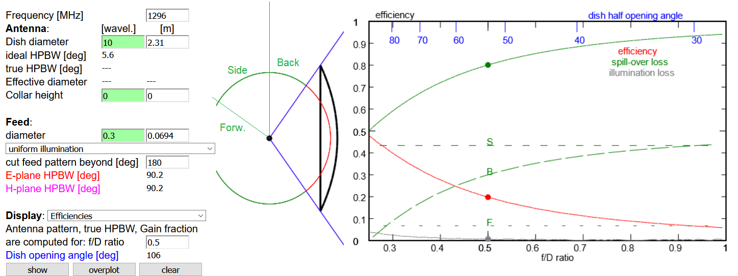
Sometimes, several green curves are present, as in this example of an isotropic feed. They show the spill-over loss in more detail:
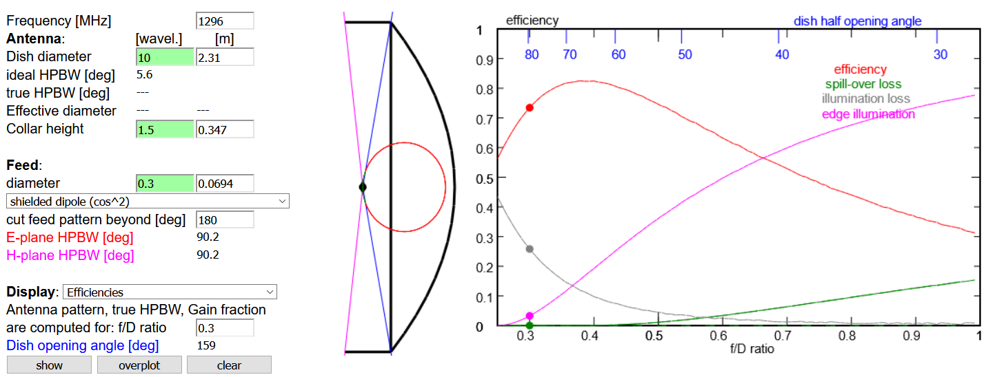
One may also investigate the effects of a conductive collar at the dish edge. This cuts down the spill-over from the rear of the antenna, and therefore reduces the noise.
Also, a magenta curve gives the illumination at the edge of the dish. This is in linear units, so that the usually recommended value of -10 dB corresponds to 0.1.
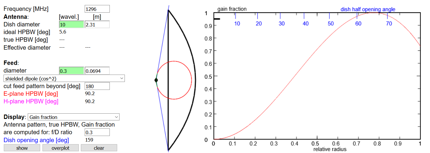
This plot shows how much each circular ring of the dish contributes to the antenna gain. One notes that the central 10 percent of the dish provide only a small amount to the gain, much less than a ring with a width of 10 percent of the dish radius. The reason is the difference in surface area of each part. The small horizontal black bar near the left top indicates the geometric obscuration by the size of the feed.
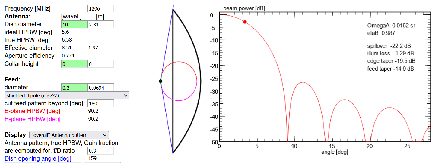
The far-field radiation patterns (in the E-plane or H-plane; the "overall" view assumes as feed amplitude the mean of E and H plane values, as used for the calculation of efficiencies) are computed for the chosen configuration of the antenna. This may take a few seconds, before the curve is displayed. The red dot marks the true HPBW whose value is also displayed on the left hand panel, along with the effective diameter of the dish. This is the diameter of a uniformly illuminated circular dish which gives the same HPBW as the chosen antenna. The aperture efficiency is the ratio of the effective and the geometrical area of the dish (i.e. the ratio of the squares of effective and geometrical diameters). In this example it is 72%.
Several parameters are displayed: the antenna solid angle ΩA, the beam efficiency ηB = ΩB/ΩA, spillover, illumination loss, edge and feed taper.
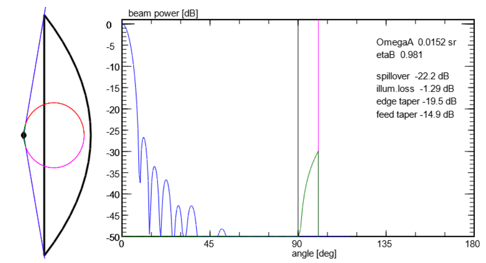
A second plot shows the far-field radiation pattern for the entire hemisphere, together with the spill-over contribution as the green curve. The vertical black line at 90° indicates the border between the forward beam (left) and the backward side of the antenna. It also displays the beam efficiency factor which is the fraction of the forwardly radiated power that is in the main beam, thus a measure of the (un)importance of the sidelobes.

When you change a parameter, such as the diameter of the feed, hit the enter key and the plot will be updated with the new data. In this way you can explore how the parameters influence the results.
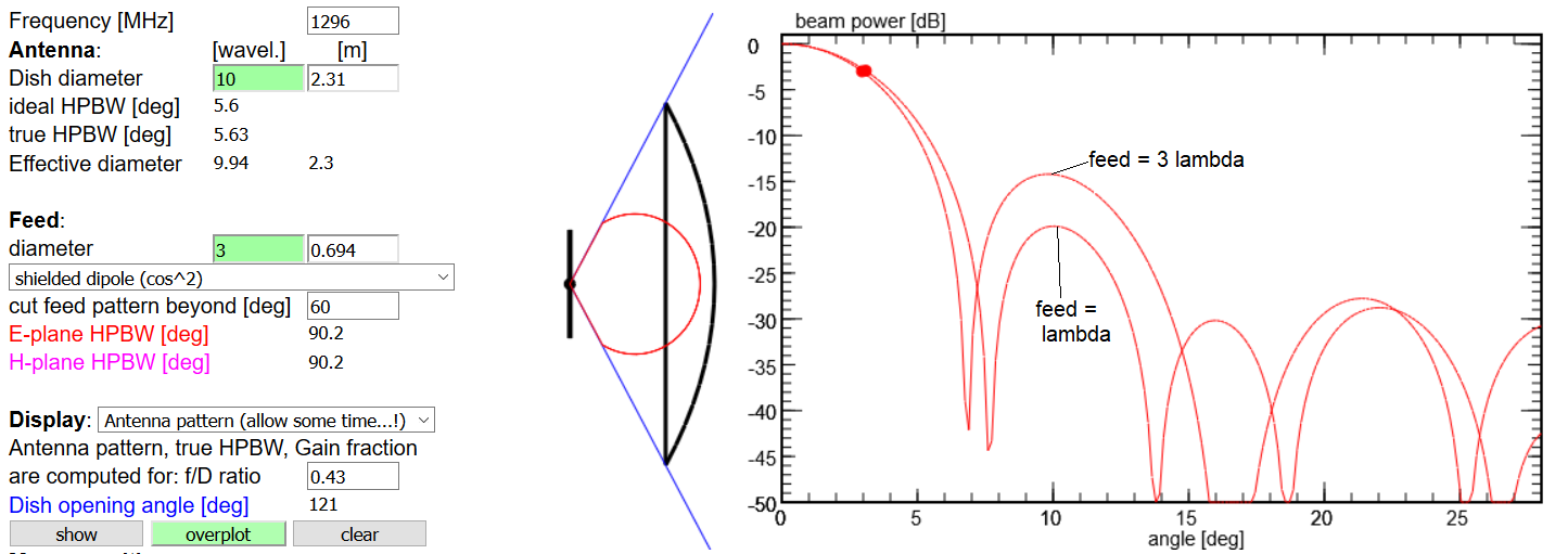
Normally, a change of parameters will clear the plot to show the current version. Click the button overplot. As long as it has a green colour (and is active), the curves from all following models are superposed. This allows you to compare directly how different values for a parameter change the results. If you take a screenshot, you may want to edit that image file (with "Paint") to mark the different curves with their associated parameters, as shown in the above picture. Once the plot gets too cluttered up with curves, use the button clear to wipe all curves.
How to start ...
In all operations on the Compute & Display page, we first give the Frequency and the Dish diameter of the antenna. We may specify the diameter in wavelengths or in meters. Hit the enter key after you entered the number in the chosen field, to make this field green to confirm your choice.
Then you will find below the ideal HPBW, which is for an uniformly illuminated circular dish. The true HPBW and the effective diameter are computed and displayed only when you had chosen to display the antenna pattern.
Then you give the parameters of the Feed: Specify its diameter (we assume that it is of circular shape, too), and choose among a list the type of feed. This list contains:
- several theoretical patterns, from a uniform illumination to various more focussed patterns. The screenshot shows that of a simple dipole whose radiation is shielded towards the outside
- measured or simulated feeds from W1GHZ: waveguides, horn antennas, helical feeds, and others
- read the data from Input page: here you enter the feed pattern in a text area at Input: Feed Pattern, following the example given there. It is the same syntax as in W1GHZ files.
- read the data from User computer: When this option is chosen, a button Browse... appears at the top of the page. Clicking this will open a file selector menu on your computer, with which you select your file. Note that your file must be a text file, conforming to the format given in the example on Input: Feed Pattern!
The HPBWs in the E-plane and the H-plane are displayed. Note that some patterns are only given in the E-plane, including the data from the Input page or from the User computer!
The sketch left of the plot shows the true geometry of the antenna and feed, with the feed pattern (red curve) and the opening angle of the dish as seen by the feed (blue lines).
Common to all plots is the display of the current coordinates of the computer mouse, which are displayed at the lower left corner.
Next, chose the Display:
... view the Feed Pattern
The plot shows the pattern of the feed antenna: if the pattern is available in both E- and H-plane, the red curve displays the E-plane pattern. Otherwise, a single magenta curve shows the feed pattern. The dot on each curve indicate the feed HPBW in the corresponding plane. The vertical blue line marks the angle to the dish's rim; thus, the power in the part of the pattern that extents beyond this angle is lost by spill over.
... view the Dish illumination
The plot shows how the illumination varies over the dish: if the pattern is available in both E- and H-plane, the red curve displays the E-plane pattern. Otherwise, a single magenta curve shows the feed pattern. The vertical blue line marks the outer rim of the dish; thus, the power in the part of the pattern that extents beyond this radius is lost by spill over.
... view the Efficiency Plot
This plot shows the same quantities as the plots in Paul's book, as functions of dish f/D ratio. The red curve is the feed efficiency, i.e. the fraction of the power fed to the antenna which is actually radiated into the antenna beam and thus in the desired direction. Like in Paul's program, this and the other quantities are computed by taking the mean of the E- and H-plane amplitudes at each angle as the amplitude which illuminates the dish. The green curve shows the spill-over loss, i.e. the fraction of feed power that is radiated beyond the dish's outer rim, and thus is not available for being focussed into the antenna beam. The grey curve is the illumination loss which is a measure of how much the dish differs from the ideal of fully illuminated antenna. The dots in the curves mark the currently chosen f/D ratio, as shown on the left hand panel. Blue marks indicate the half opening angle of the dishes as a function of f/D ratio.
Please note that this feed efficiency is neither the aperture efficiency which is the fraction of the radiated power of what could be radiated by a uniformly illuminated dish nor what may be called the overall efficiency which would include the beam efficiency. Any other effects, such as scattering due to surface irregularities and ohmic losses, would further need to be taken into account.
Sometimes, several green curves are present, as in this example of an isotropic feed. They show the spill-over loss in more detail:
- A curve with long dashes is the spill-over to angles higher than 90° from the main beam, and thus towards the rear of the dish. This is important because of the pickup of thermal noise from the ground.
- Shorter dashes are the spill-over to the sides, to angles between 30 and 90° off the main beam. Usually this is not too important if there are no high trees or buildings block the sight.
- Very short dashes is the spill-over to the front, within 30° of the main beam. Obviously this is of little importance, as one would pick up noise from the sky.
- The full line is the total spill-over, i.e from all directions.
One may also investigate the effects of a conductive collar at the dish edge. This cuts down the spill-over from the rear of the antenna, and therefore reduces the noise.
Also, a magenta curve gives the illumination at the edge of the dish. This is in linear units, so that the usually recommended value of -10 dB corresponds to 0.1.
... view the Gain Fraction
This plot shows how much each circular ring of the dish contributes to the antenna gain. One notes that the central 10 percent of the dish provide only a small amount to the gain, much less than a ring with a width of 10 percent of the dish radius. The reason is the difference in surface area of each part. The small horizontal black bar near the left top indicates the geometric obscuration by the size of the feed.
... view the Antenna Pattern
The far-field radiation patterns (in the E-plane or H-plane; the "overall" view assumes as feed amplitude the mean of E and H plane values, as used for the calculation of efficiencies) are computed for the chosen configuration of the antenna. This may take a few seconds, before the curve is displayed. The red dot marks the true HPBW whose value is also displayed on the left hand panel, along with the effective diameter of the dish. This is the diameter of a uniformly illuminated circular dish which gives the same HPBW as the chosen antenna. The aperture efficiency is the ratio of the effective and the geometrical area of the dish (i.e. the ratio of the squares of effective and geometrical diameters). In this example it is 72%.
Several parameters are displayed: the antenna solid angle ΩA, the beam efficiency ηB = ΩB/ΩA, spillover, illumination loss, edge and feed taper.
... view the Antenna Pattern including Spill-Over
A second plot shows the far-field radiation pattern for the entire hemisphere, together with the spill-over contribution as the green curve. The vertical black line at 90° indicates the border between the forward beam (left) and the backward side of the antenna. It also displays the beam efficiency factor which is the fraction of the forwardly radiated power that is in the main beam, thus a measure of the (un)importance of the sidelobes.
... play with parameters
When you change a parameter, such as the diameter of the feed, hit the enter key and the plot will be updated with the new data. In this way you can explore how the parameters influence the results.
... compare different models
Normally, a change of parameters will clear the plot to show the current version. Click the button overplot. As long as it has a green colour (and is active), the curves from all following models are superposed. This allows you to compare directly how different values for a parameter change the results. If you take a screenshot, you may want to edit that image file (with "Paint") to mark the different curves with their associated parameters, as shown in the above picture. Once the plot gets too cluttered up with curves, use the button clear to wipe all curves.
E-plane:
H-plane:
Frequency [MHz]
Antenna: [wavel.] [m]
Dish diameter
ideal HPBW [deg]
true HPBW [deg]
Effective diameter
Aperture efficiency
Collar height
Feed:
diameter
cut feed pattern beyond [deg]
E-plane HPBW [deg]
H-plane HPBW [deg]
Display:
Antenna pattern, true HPBW, Gain fraction
are computed for: f/D ratio
Dish opening angle [deg]
Mouse position