- Basic Explanations
- A Walk thru the Tool
- Compute & Display
- Input: Feed Pattern
- Outputs: Ant.Pat. or Fillfactor
Filling Factors For Antenna Patterns
Joachim Köppen DF3GJ ... Kiel, Dec. 2020
Some brief explanations
- This tool computes the dependence of the beam filling factor on the ratio of object diameter (FWHM) and antenna HPBW. This factor is defined as the ratio of the power received by the antenna from the object and the power picked up by the antenna if the object were evenly bright and large enough to fill the entire antenna beam.
- While one could compute it for any position of the antenna beam and the object,
it is commonly given for the antenna beam well centered on the object,
both being supposed to be of circular shape. Then the fill factor is
given by:
fill = ∫ A(r) * (O(r)/O(0)) 2π r dr
with the antenna pattern A(r) which is normalized as:
∫ A(r) 2π r dr = 1
and the object's brightness profile O(r). The integration is in the radial distance from the beam centre, extending from r = 0 to any distance large enough to cover the entire antenna pattern and the object's profile. Because of the circular shapes the angular integration amounts only to the factor 2π. - Note that these functions are the 2-D distributions, so
that a gaussian antenna beam is given by:
A(r) = exp( -r²/2σ² ) / (2πσ²)
with HPBW = 2 √(2 ln2) σ = 2.3548 σ - A large source of uniform brightness has the filling factor 1,
but a source much smaller than the antenna beam has a small filling factor.
For the primitive example of a tophat object (= disc of constant brightness)
and a tophat antenna beam (= constant sensitivity up to the rim), the
filling factor is equal to the ratio of the angular areas:
fill = 1 for FWHM ≥ HPBW
fill = (FWHM/HPBW)² for FWHM ≤ HPBW
... or written more compactly : fill = max(1, (FWHM/HPBW)²)
- After inputing a value in one of the text fields, hit the Enter key to show the new plot.
- The computation of non-uniform illumination patterns may take some time! Because it seems not possible to indicate when the tool is busy, be patient.
- The mouse position gives the coordinates of that point, allowing to read numerical values from the plot. In some browsers, these values may not correspond to the plot. If this happens, keep this page in its initial top-left corner position.
- Please note that due to the finite accuracy chosen to get reasonably fast computations, some curves may show some small irregular wiggles...
- The antenna pattern can be selected among:
== Beam shape: tophat, gaussian shape for the main lobe
== Square: a few patterns from a square antenna, illuminated in a few simple ways
== Circular: a few patterns from circular dishes, illuminated in a few simple ways
== Feed: circular dish illuminated by feed patterns, at specified f/D ratio == == simple feed patterns == == feed patterns input by the user from either the Input Page or the user's computer == == feed patterns from the W1GHZ antenna book - Source patterns can be chosen as:
== tophat: uniformly bright disc
== gaussian disc: has width FWHM, but extends beyond this point
== disc (radius FWHM/2) with limb darkening: a gaussian which has the specified level (≤ 1) at the outer rim
== == ditto, but with cos0.2(latitude) from Krotikov & Shchukov (1963)
== == ditto, but with cos0.5(longitude) from Krotikov & Shchukov (1963)
== == ditto, but for limb brightening (or darkening), following r6 which gives the specified level at the outer rim - After choosing antenna and source patterns, click on the appropriate green botton:
- The Antenna and Source Patterns are shown by three curves as
a function of offset angle in units of the (fixed) antenna HPBW:
the antenna pattern is in blue, grey is the source brightness profile,
and red is the source pattern as smoothed by the antenna beam.
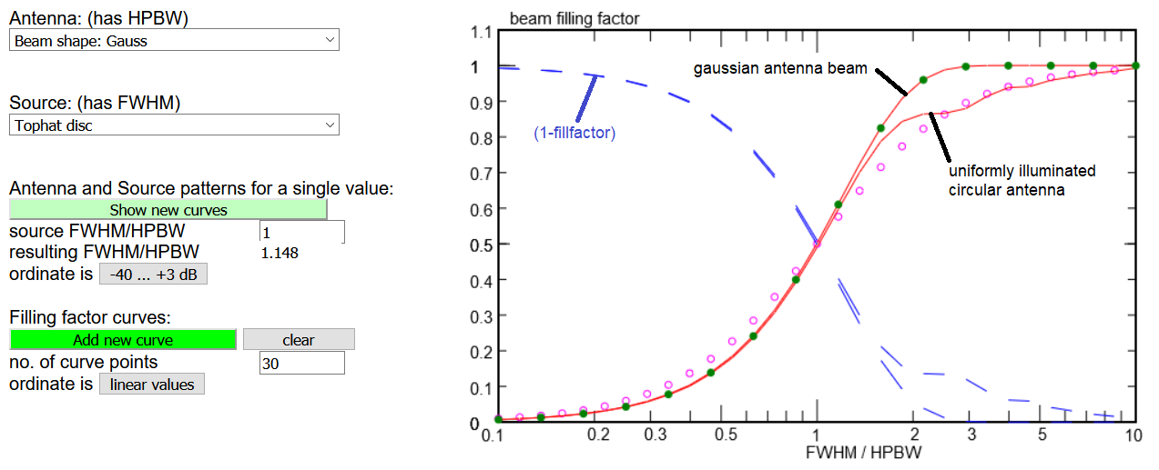
- The filling factor (red curve) is displayed as a function of the ratio x = FWHM/HPBW of the angular widths of source and antenna beam, respectively. In the plot with linear ordinates, a blue dashed curve is (1-filling factor) shown for convenience, as this amounts to the fraction of noise from the surrounding sky area.
- In the filling factor plot a new curve is superposed on existing ones. This feature allows easier comparisons, but makes it necessary to clear manually the plot whenever it is felt necessary.
- The small magenta circles are the approximation for a Gaussian antenna beam looking at a circular object with Gaussian brightness distribution: filling factor = x²/(1+x²). This simple expression is quite a useful approximation.
- For a Gaussian antenna beam and a uniformly bright disc (tophat), the green dots are from the formula by UA3AVR: filling factor = 1-2-x*x [eq. 4b in DUBUS 3/2016, p.34]
| Top of the Page | Java Applets Index | JavaScript Index | my HomePage |

When you selected the shapes of the antenna beam and the source, and put in a value for the
ratio of source FWHM and antenna HPBW, a click on the button 'Show new curves' will display
the brightness profile of the source (in grey), the antenna beam (blue), and that of the image
obtained with this antenna (red). Since here the two widths are comparable, the image is a little
wider.
If you enter another value for the source size, hit the enter key to display the new curves.
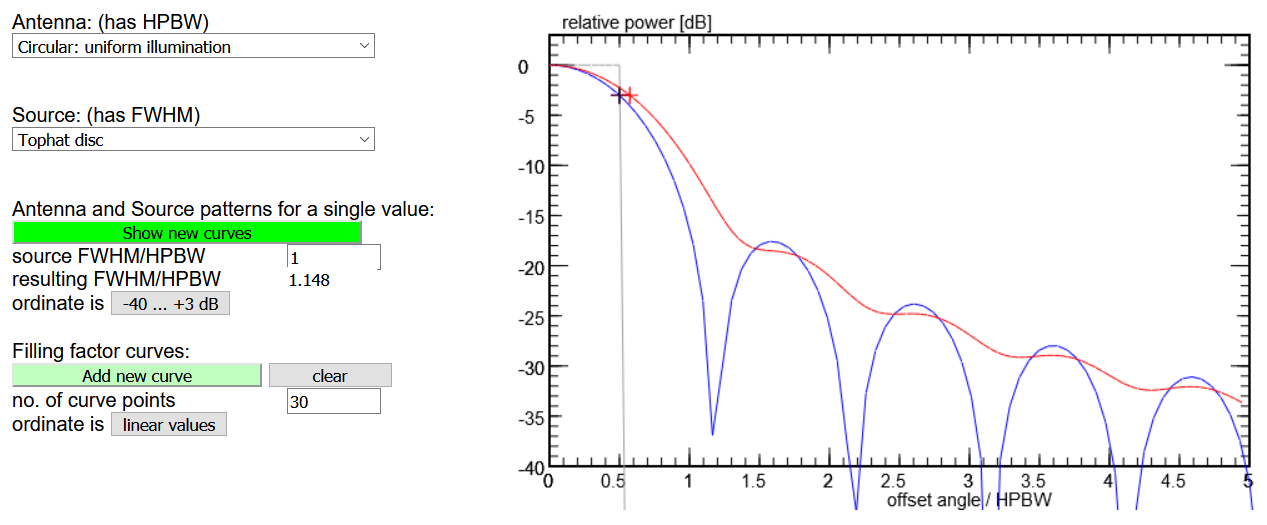
The sidelobes of the antenna pattern are not very visible in a plot with linear ordinates.
With logarithmic or dB scales they become much more prominent.
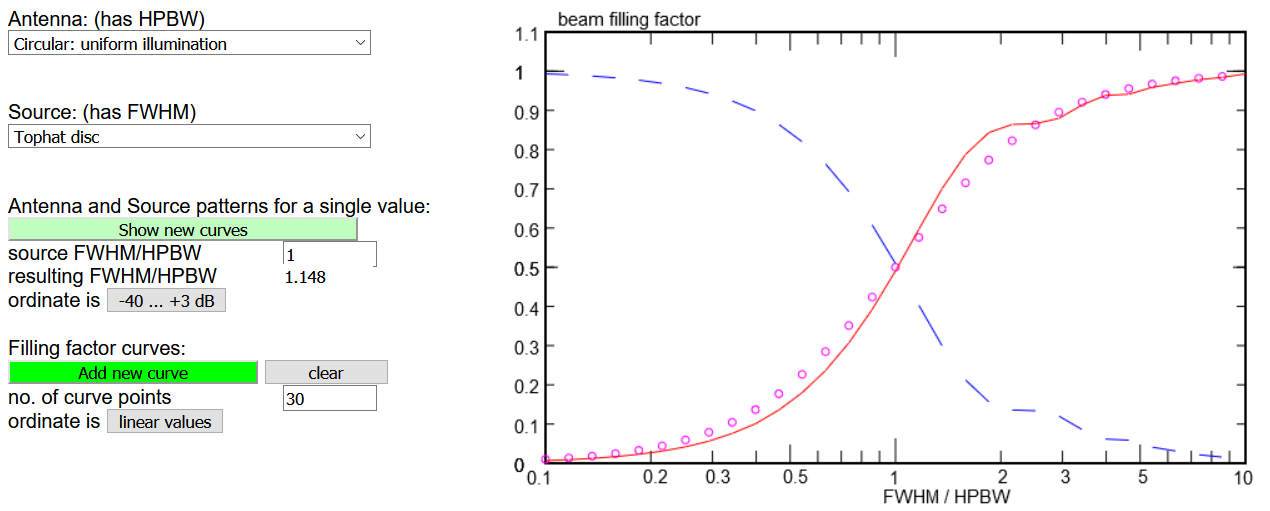
When we want to see for this antenna/source combination the filling factor as a function of the
ratio x = FHWM/HPBW, we click the lower button 'add new curve'. It shows the result as a red curve,
with small magenta circles indicating the simple approximation x²/(1+x²) which
is strictly valid for a gaussian source and a gaussian antenna beam. The dashed blue curve is
(1-fillfactor) which indicates how much of the background around the source would be picked up
by the antenna.
To compare with another configuration, click the 'add new curve' again to superpose the new results.
Use the 'clear' button when the plot becomes too cluttered.
Next, let us use the pattern of a circular antenna which is illuminated by a feed antenna, whose
pattern had been measured. This pattern can be input directly in the text area under the tab
'Input: Feed pattern':
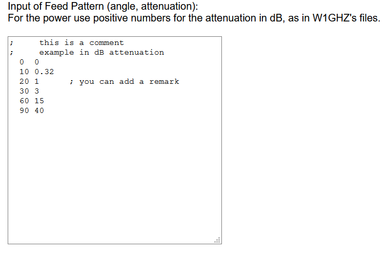
The format is the same as in the files of W1GHZ: angle and attenuation in dB.
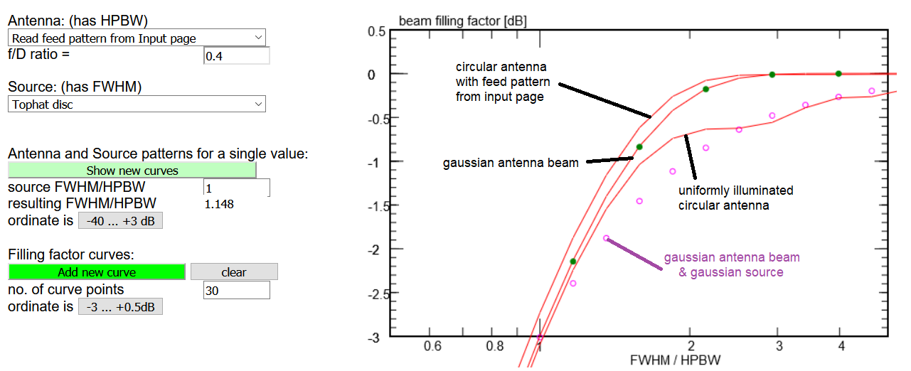
Choose as antenna: Read feed pattern from Input page ...
... if you click 'Show new curves' the antenna pattern is displayed, but if
you want to see directly the filling factor function, click the 'add new curve' button.
In the above image - done with a zoomed view of the plot - we already had computed some
other configurations to compare with it: Here it appears that the antenna pattern is
quite close to a gaussian function.
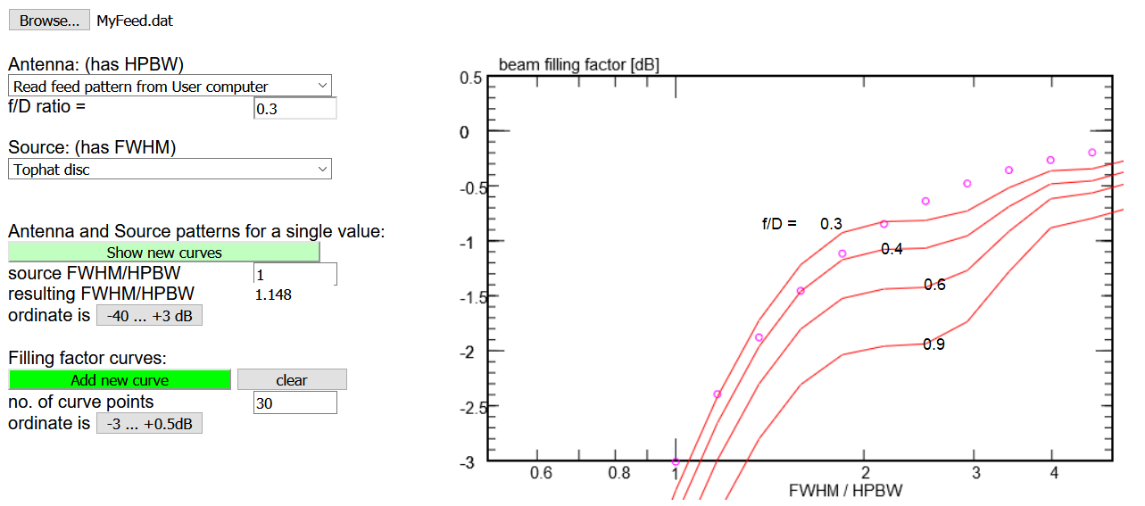
You may also enter a feed pattern from a text file on your computer: The format of the text file
is the same as in the files of W1GHZ: angle and attenuation in dB. As described under the
'Input: Feed Pattern' tab. Reading the file is done by choosing as antenna
Read feed pattern from User computer.
A button 'Browse...' appears; click it to open a file selection menu ...
In the above image we explored how this feed behaves when illuminating dishes with different
f/D ratios. It appears to be better suited for deep dishes with f/D = 0.3..0.4.
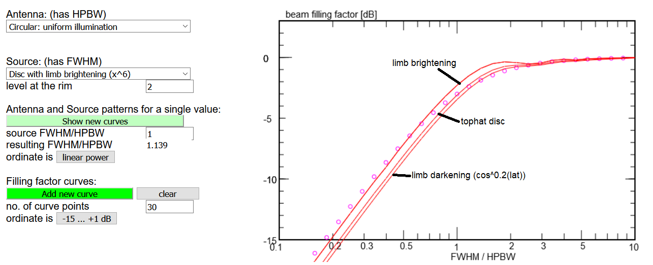
All above examples were done with a tophat source, i.e. whose brightness is constant over
the entire face. As the radio Moon is brighter in the middle than near the rim, there are
three recipes to describe this limb darkening: the brightness follows a gaussian function
and has a certain value at the rim, or it follows cosine laws, which Krotikov &
Shchukov (1963) found for the latitude and longitude dependence. Similarly, the radio Sun
is brighter near the rim than in the middle, because of the emission by the very hot corona.
This limb brightening is described in a simple and crude way: assuming that the brightness
increases like the sixth power of the radius and reaching a specified value at the rim.
The plot above explores how the deviations of the source brightness profile from the simple tophat
influence the filling factors.