Stellar Population
Joachim Köppen Kiel Dec 2018
Some brief explanations
The luminous matter in the Universe is organized in galaxies which consist of stars and interstellar gas. The stars have been born at various times in the past from the gas by cold molecular clouds becoming unstable against their own gravity. Nearly all the optical brightness of a galaxy comes from the present stellar population which thus may be a combination of young and old, hot and cool stars. From theoretical work, it is fairly well known how stars of the various masses change with time, so it is possible to model a population of stars, in order to find out how star formation occurred in the past. Because star formation is something we still cannot derive from basic physics, one describes this process by assuming that stars are born following a certain distribution Function of their Initial Masses (the IMF, usually decreasing like a power law with increasing mass), and that the star formation rate (SFR) describes how much gaseous matter is converted per time unit into any kind of stars. The evolution of the new stars depends on the metallicity of the gas out of which they were formed.
This tool permits the user to compute the theoretical and observable properties of single stars of any mass and age and various metallicities. It also permits to create synthetic populations of stars born with any arbitrary history star formation.
There are three principal pages:
- Stars & Evolution: Here one can explore how the properties of a single star, such as its temperature, luminosity, and photometric colours change with its mass, age, and metallicity. For a given stellar mass the evolutionary tracks can be displayed, as well as for a given age the isochrone curves can be plotted.
- Star Formation History: Here the user specifies how the star formation rate changes with age, and also gives other parameters necessary for the simulation of a stellar population.
- Synthetic Population: computes the properties of the stars of such a simulated population, based on the user-defined star formation history. It displays the data in a Hertzsprung-Russell diagram or Colour-Magnitude diagrams.
The theoretical evolutionary tracks of stars between 0.8 and 120 solar masses are from the computations of the Geneva group (C.Charbonnel, A.Maeder, G.Meynet, D.Schaerer, G.Schaller (1992ff) Astron.Astrophys.Suppl. 96, 296; 98, 523; 101, 415; 102, 339). The tables for the photometric colours in the Johnson UBV system were computed by G.Lapierre (Strasbourg) with the Kurucz' grid of theoretical stellar spectra.
The controls on the Stars & Evolution page are:
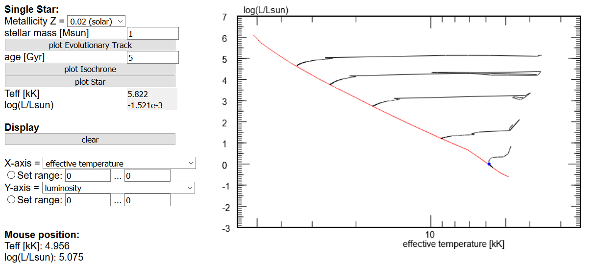
- Metallicity: specifies the abundance of the elements heavier than helium (AKA 'metals') in the gas matter of the star. The quantity Z is the mass fraction of these elements. Solar composition is Z=0.02. A choice of 5 values are given, from metal-poor stars (Z=0.001) to twice solar composition (Z=0.04).
- stellar Mass: the user specifies the mass of the star at the beginning of its life on the main sequence.
- Evolutionary Track: a click will plot the evolutionary track (as a black curve) of the star with the given mass, from the start on the main sequence to the end of the evolution on the red giant branch.
- age: the user gives the age of the star, i.e. the time since the star started on the main sequence.
- Isochrone: a click plots in any diagram the location of stars of all masses but of the same age, as a red curve.
- Star: a click plots the position of the star with given mass and age, as a small blue dot.
- Teff and log(L/Lsun): are the effective temperature and luminosity of the displayed star.
- clear: wipes all curves on this plot. Note that each click of the buttons adds the corresponding curve to the plot.
- X-axis, Y-axis: chooses the two parameters for the plot:
- effective temperature
- luminosity
- mass
- radius
- surface gravity
- age (linear scale), age (log scale)
- U, B, V: absolute brightness in the bands of about 365, 440, and 548 nm wavelength.
- U-B, B-V: the colour indices
- mU, mB, mV: apparent brightness in the bands of about 365, 440, and 548 nm wavelength.
- mU-mB, mB-mV
- Set range: enter the values for the range to be displayed, then click the radio button, to show the plot with the requested ranges. Avoid entering 0 or a negative value when the parameter is a logarithmic quantity.
- Mouse position: displays the coordinates of the present position of the mouse.
The controls on the Star Formation History page are:
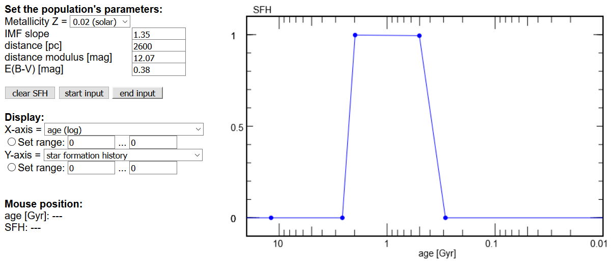
- Metallicity: specifies the abundance of the elements heavier than helium (AKA 'metals') in the gas matter of the star. The quantity Z is the mass fraction of these elements. Solar composition is Z=0.02. A choice of 5 values are given, from metal-poor stars (Z=0.001) to twice solar composition (Z=0.04). This choice is always consistent with the same control on the Stars & Evolution page.
- IMF slope: is the exponent of the Initial Mass Function, i.e. the distribution of the stellar masses at their beginning on the main sequence. Here we use a simple power law, with the exponent 1.35 being approximately appropriate for the Milky Way.
- E(B-V): specify the colour excess to take into account the interstellar reddening towards an observed object. Otherwise, use 0
- distance, distance modulus: specify either value when you want to compare simulation results with observational data. Click on the field to make it input (light green colour), enter the value and hit the Enter key. The other value then is computed and displayed.
- clear SFH: clears this plot and also any previously entered history.
- start input: click this, so that you can click on the plot to graphically
enter a history. Each click adds a blue dot to the plot, joined with a straight
blue line to the previous dot. To move a dot, click on it and drag it to the
desired position. A series of blue circles will trace the path, but will disappear
when the dot is released at the new position.
Note: when a dot is placed or moved to a negative values of the SFH, it will be set to zero, i.e. no star formation.
Note: the SFH is taken constant before the first dot and after the last dot. - end input: click this to exit the input mode and to display the final version of the entered SFH.
- X-axis: one may choose between a linear or logarithmic scale for the age
- Set range: enter the values for the range to be displayed, then click the radio button, to show the plot with the requested ranges. Avoid entering 0 or a negative value when the parameter is a logarithmic quantity.
- Mouse position: displays the coordinates of the present position of the mouse.
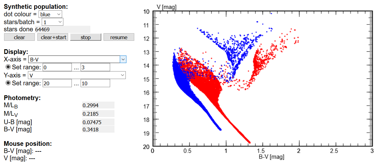
The controls on the Synthetic Population page are:
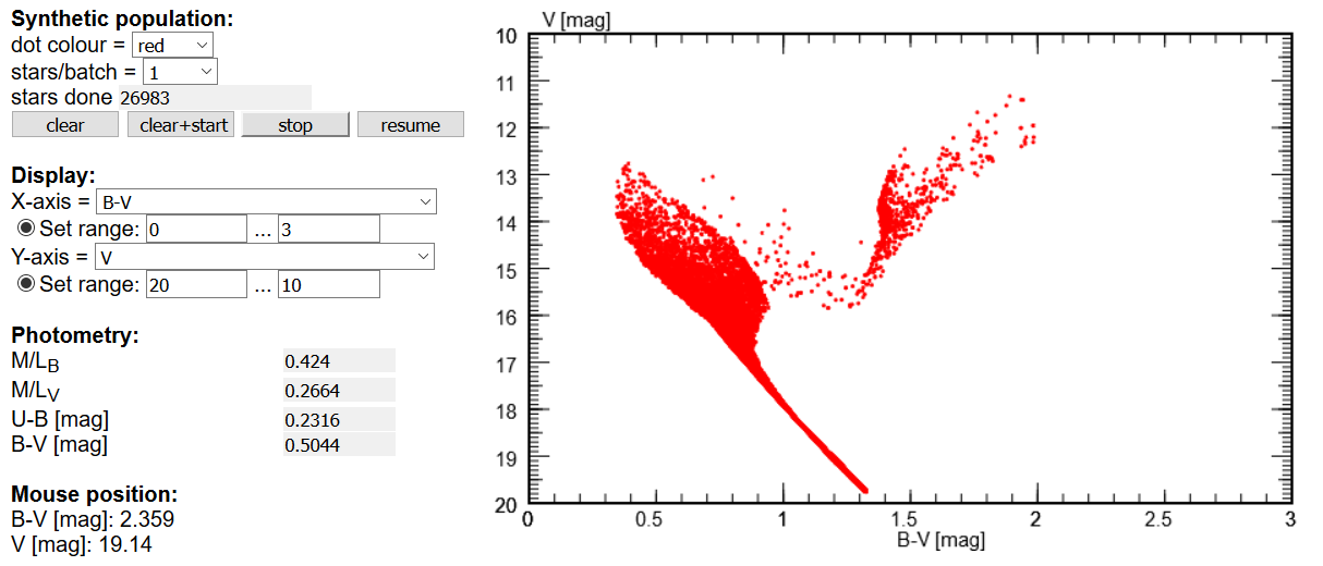
- dot color: chooses the colour of the dots which represent a star in the plot.
- stars/batch: is the number of stars generated by each call of the simulator section. If one wants to see quickly the results for a large number of stars, one may choose a high number (However, with a huge population, a few computational artefacts caused by e.g. the interpolation of data become more visible ... do not overinterpret the presence of such fine features!)
- stars done: displays the total number of stars generated so far.
- clear: wipes the plot
- clear+start: starts a new simulation, clearing all previous results.
- stop: halts the current simulation.
- resume: continues with the simulation. Note that any changes in the parameters (metallicity, IMF, star formation history, ...) are taken into account. In this manner, one may create a mixture of populations of stars with different SFHs.
- X-axis, Y-axis: chooses the two parameters for the plot, as on the Stars & Evolution page. Note that when changing parameters, the plot is wiped, and one simply repeats the simulation.
- Set range: enter the values for the range to be displayed, then click the radio button, to show the plot with the requested ranges. Avoid entering 0 or a negative value when the parameter is a logarithmic quantity.
- M/LB and M/LV: display the ratio of stellar mass and luminosity in the B- and V-band of the entire stellar population.
- U-B, B-V: display the colour indices of the entire stellar population.
- Mouse position: displays the coordinates of the present position of the mouse.
| Top of the Page | Java Applets Index | JavaScript Index | my HomePage |
How to ...
- ... compute isochrones and evolutionary tracks
- ... compute the population of stars born ...
- ... add a second population of metal-poor stars